ORIGINAL ARTICLE
PASQUALI, Guilherme [1], NASCIMENTO, Vagner do [2]
PASQUALI, Guilherme. NASCIMENTO, Vagner do. Failure analysis and fatigue life of a centrifugal fan drive shaft. Revista Científica Multidisciplinar Núcleo do Conhecimento. Year. 07, Ed. 09, Vol. 02, p. 115-139. September 2022. ISSN: 2448-0959, Access link: https://www.nucleodoconhecimento.com.br/engineering-mechanical-engineering/centrifugal-fan
ABSTRACT
This article represents a numerical analytical study of the drive shaft of an industrial exhaust fan, which failed due to fatigue in the work field and required its replacement. The main objective of this work was to identify the region of stress concentration and quantify the time/number of cycles that the part took to failure. With this, all the mechanical stresses involved in the operation of a centrifugal fan were calculated, in order to obtain bending moment, shear and axial force in the component. Analytically, the region of greatest static mechanical stress was evident, with a great sensitivity to notch that leads to mechanical fatigue. Subsequently, numerical analysis by finite elements corroborated the calculations and confirmed the number of cycles and the fatigued region in operation, with a relative error of only 5%.
Keywords: Centrifugal fan, Drive shaft, Fatigue, Finite Elements.
INTRODUCTION
The constant advancement of engineering development technologies has increased access to tools and knowledge for problem solving in the industry. The use of the finite element method has been used to shorten steps, validate calculations and sometimes identify divergences and incongruities in the analytical work of the engineer.
Such tools are valid and also of interest when it comes to the design of industrial centrifugal fans. Machines that continuously provide energy to a given fluid, in order to overcome the resistance generated by piping and components, reaching the flow point demanded by the process to which it is involved.
For Bleier (1997), a combination of the use of centrifugal force to move the air in the radial direction with the deflection of the air flow by the rotor blades.
According to Jorgensen (1999), an equipment that generates a constant current of air through the rotating movement of an impeller mounted on an axis.
Object of study of this work, for Gujaran and Gholap (2014), transmission shafts are used to transmit power and/or torque through gears, pulleys, keys, clutches and sprockets.
In addition to static loads, the shaft is subjected to a series of dynamic loads that can lead to fatigue failures, according to Roy et al. (2020). For Zambrano (2014), fatigue is the most common cause of problems with rotating machinery shafts, usually at points of stress concentration and keyways.
Since the purpose of this work is to elucidate, analytically and numerically, how an axis responds to the mechanical demands imposed by the operation of a flow machine, stresses were methodically estimated and analysis points selected for fatigue calculation.
Trebuna et al. (2009), demonstrated that fatigue failure can occur in an axis due to the equipment operating frequency being very close to the natural frequency of the machine structure. Poorly dimensioned mechanical structures can amplify mechanical excitations and anticipate failures.
The drive shaft, according to Jorgensen (1999), when subjected to fan operation, undergoes mechanical tensions, compressive, torsional and bending moments that can act alone or even in combination. For Norton (2004), with this the shaft can experience completely alternating stresses, considering the presence of bending moment on the component; and that the combination of this bending moment and a torque creates complex multiaxial stresses.
Geralmente eixos não possuem diâmetro uniforme, mas sim reduções, chavetas, cantos agudos entre outros. A tensão no eixo em um ponto específico varia de acordo com a rotação levando a fadiga. Mesmo um componente perfeito quando submetido repetidamente a carregamentos de magnitude suficiente, pode eventualmente propagar uma trinca de fadiga em uma região de alta tensão, geralmente iniciando na superfície até que a fratura ocorra. (GUJAR; BHASKAR, 2013, p. 1061).
Ristivojevic (2010) details that in addition to the known shaft tension concentrators, items such as bearing adapter sleeves can undergo dimensional changes due to temperature variations and cause mechanical interference during operation.
Callister (2002) mentions that a fatigue failure is fragile in nature, even in high ductility metals, given the low or almost non-existent plastic deformation. The process takes place by the initiation and propagation of cracks and usually the surface of this crack is perpendicular to the direction of stress generated by traction.
The study details an axis that failed due to fatigue during its operation, seeking to correlate the analytical calculations and the theory, together with the simulations to understand which critical regions are and how to prevent them, considering the boundary conditions specified below. At the end, the results are compared together with the practical effects and what happened in the equipment.
MATERIALS AND METHODS
In order to understand the efforts on an industrial centrifugal fan shaft, it is necessary to characterize the equipment and the operating conditions, in order to quantify and identify each of the requests in a coherent way.
The machine in question is a large extractor with 400hp of power, with flow, static pressure and shaft rotation of respectively 300,798m³/h, 290 mmCA and 590 RPM.
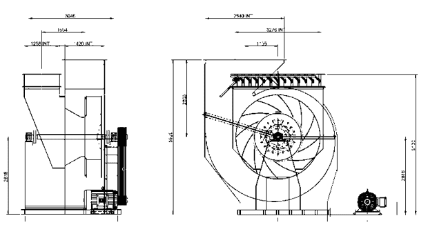
Figure 1: 400 hp bi-supported shaft exhaust
It is also important to know the rotor inlet and outlet diameters and heights. Armed with this information, it is possible to start calculating the requests generated on the axis.
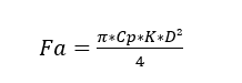
Jorgensen (1999), indicates that the calculation of the axial force on the shaft due to the pressure differential is done through Equation 1.
 (1)
(1)
Cp being the conversion factor 9.79 (Pa/mmH20); K the proportionality constant, which in this case is 1; p is the total pressure of the equipment (mmH20) and D is the rotor diameter.
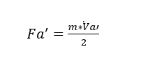
The change in the direction of the air flow also causes axial force on the axis which, according to Jorgensen (1999), is calculated according to Equation 2.
 (2)
(2)
Where ?̇ is the mass flow rate (kg/s); Va’ is the axial velocity of the fluid (m/s) and g is the acceleration due to gravity (m/s²).
For Henn (2006), the operation of a fan generates radial force on the shaft, while it does not operate exactly at the design point at which it was dimensioned. Equation 3 illustrates how to calculate it.
![]()
(3)
Where Kf is the coefficient that varies according to the impelled flow and is calculated by Equation 4; ? is the specific mass of the fluid (kg/m³); Y is the energy jump (J/kg); D is the rotor diameter and b5 is the rotor outlet width (m).
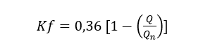
(4)
For Equation 4, Q is the flow rate driven by the machine and Qn is the nominal flow rate determined in the design.
It is known that there is no possibility of manufacturing a perfectly balanced rotating machine, according to Jorgensen (1999), there will always be excitation forces at a frequency proportional to the operating rotation of the equipment. For Shahrooi and Asayesh (2013), an unbalanced rotor can generate voltages up to 50% higher in the restriction regions of the shaft in relation to the rated operating voltage.
The ISO 1940:2003 Standard establishes degrees of balancing quality according to the type of equipment and mode of application. Having defined the Quality Degree for centrifugal fans, having in hand the operating rotation, it is possible to determine the maximum specific unbalance mass for a rotor, through the graph in Figure 2.
Figure 2: Specific unbalanced mass table. ISO 1940
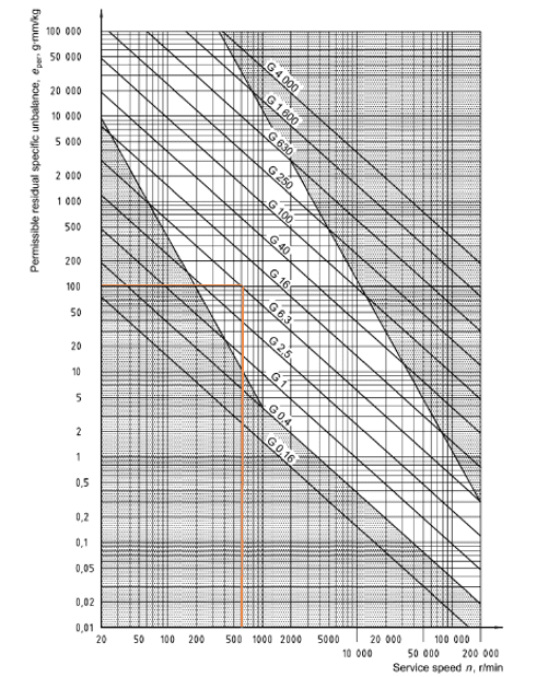
With this, it is possible to determine the residual unbalance mass and adopt the highest value allowed by the Standard to calculate the centrifugal force.
Nishi (2006) cites that the residual mass can be calculated according to Equation 5.
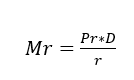
(5)
Where Mr is the residual mass, Pr is the rotor weight (kg), D is the specific unbalance mass found in the table (g.mm/kg) and r is the rotor radius (mm).
Assuming that this unbalanced mass is located close to the outer diameter of the rotor, the centrifugal force can be determined according to Equation 6.
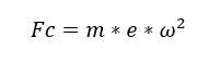 (6)
(6)
Where m is the unbalanced mass (kg), “e” is the eccentricity of the mass (m) and w is the radial velocity (rad/s).
Another important consideration to be made, arising from machine designs, is to estimate the force exerted by the stretching of the belts, as shown in Figure 3.
Figure 3: Schematic of pulleys and belts
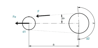
The first step to calculate the belt tensioning stress is to determine the angle g, through Equation 7.
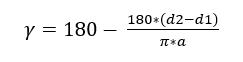 (7)
(7)
Where “a” is the distance between centers (mm), d2 is the diameter of the largest pulley (mm) and d1 is the smallest one (mm).
Whereas angle b is half of 180 minus ![]() . Another important Equation is Equation 8, for determining the tangential force on the smaller pulley.
. Another important Equation is Equation 8, for determining the tangential force on the smaller pulley.
 (8)
(8)
Where t1 is the torque (N.m) and r1 is the radius of the smallest pulley (mm). Other necessary information is the angle ![]() in radians, which will be called
in radians, which will be called ![]() .
.
The calculation of the force on the belts in the tensioned part and in the slack part of the belt is defined respectively by Equations 9 and 10, where ![]() is the average friction coefficient between belt and pulley.
is the average friction coefficient between belt and pulley.
(9)
 (10)
(10)
The total stretching force which the shaft is under the influence of is estimated by Equation 11.
 (11)
(11)
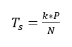
Another important stress suffered by the shaft during the fan operation is the torque, which according to Jorgensen (1999) is defined by Equation 12.
 (12)
(12)
Where K is a coefficient defined by 1000/2 ![]() , P is the motor power (kW) and N is the shaft rotation (rps).
, P is the motor power (kW) and N is the shaft rotation (rps).
Having calculated all the loads, it is possible to draw the shear force and bending moment diagrams along the axis. With this, the critical points are defined and the moments suffered are determined.
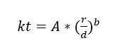
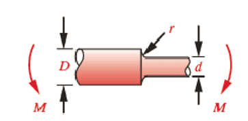
The definitions of stresses for the calculation of fatigue, need to be calculated according to Norton (2013), the sensitivity to the notch and the stress concentration factor kf, which take into account the characteristics of the material. First, however, it is necessary to estimate the geometric concentration factors kt and kts. In the case of an axle with diameter reduction, as shown in Figure 4, the type of loading must be taken into account and the factor defined according to Equation 13.
 (13)
(13)
The data required in Equation 13 are shown in Table 1.
Table 1: Data for calculating kt
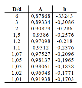
Figure 4: Shaft with reduction under moment
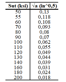
For Norton (2013), Neuber was one of the first to study the effects of discontinuities in parts and proposed an equation to estimate the stress concentration factor in fatigue. The notch sensitivity is defined from Equation 14, Kuhn-Hardrath in terms of the constant “a” and the notch radius.
The higher the material’s ductility, the lower the notch sensitivity; which also depends on how abrupt the diameter reduction is, taking into account the rounding of the diameter reduction.
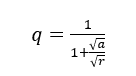 (14)
(14)
Table 2: Neuber’s constant for steels
The determination of the concentration factor kf, applied to the stress values calculated based on the previously performed mechanical stresses, is performed by Equation 15.
![]() (15)
(15)
Once the points of interest are defined, where it is estimated that there will be the highest stress points and that the shaft should fail due to fatigue, the stresses are calculated according to the type of request, see Equations 16, 17 and 18.
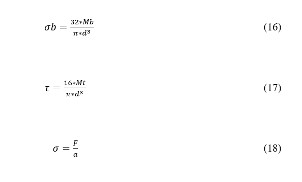
Where Mb (N.m) is the bending moment, Mt (N.m) is the torsional moment, F(N) the axial force, “a” (m²) the shaft section area and d (mm) the diameter of the selected point.
A good parameter to validate the numerical calculations with the analytical ones is to estimate the Von Mises Stress, according to Norton (2004), which is convenient in situations that combine normal and shear stresses at the same point, according to Equation 19.
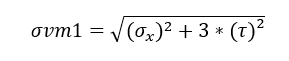 (19)
(19)
According to Hibbeler (2009), the general state of stress in a region is determined by six components of normal and shear stress. Making simplifications for a plane stress state, the maximum principal stress is determined by Equation 20.
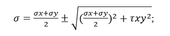 (20)
(20)
Like other mechanical properties, fatigue characteristics can be tested in the laboratory. According to Callister (2002), equipment is designed to simulate controlled loads, frequency and pattern of repetitions, in an accelerated way in order to determine how many cycles a specimen of a certain material supports under pre-established conditions.
For Norton (2004), the S-N curve has become an important way of characterizing the behavior of materials subjected to alternating stresses and is still used today. The first studies on these characteristics in metallic materials were carried out by August Wöhler in 1850, and the main result of this work was the generation of a curve that relates the number of cycles supported with the alternating stress applied to a specimen. Crack propagation studies are performed at stress levels below the strength limit and for a significant number of cycles, above 1000.
Figure 5: S-N curve with probability of failure
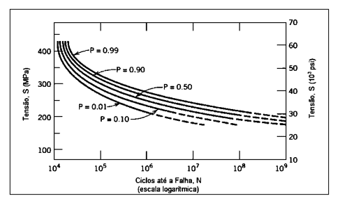
Garcia et al. (2012) cite that in general, for steels, the fatigue strength limit is between 35% and 65% of the tensile strength limit. The values obtained from tests with specimens also need to be corrected according to the actual application conditions of the projected part, whether differences in temperature, exposure environment and manufacturing method, to the point of finding the corrected fatigue strength, represented by the Equation 21.
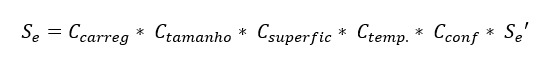 (21)
(21)
Where Se’ is 54% of the maximum voltage value for materials where Sut is less than or equal to 1460 Mpa. For values above that, Se’ is considered equal to 740 Mpa.
According to Norton (2004), Ccarreg is the correction factor for the type of loading, being 1.00 for flexion and 0.70 for normal force.
The specimens have reduced sizes, most of the times smaller than the parts under analysis, so a correction factor is applied. For diameters up to 8mm, Csize can be considered 1.00; for diameters between 8.00 and 250 mm, Equation 22 is used.
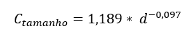 (22)
(22)
The specimen has a surface with a polished finish. Different from the designed part that suffers from imperfections, porosities, material flaws, notches, among other factors that reduce the fatigue resistance of the model.
Table 3: Surface factor coefficient
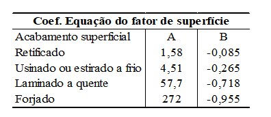
Also according to Norton (2004), to define the value of this coefficient, it is necessary to select values of A and B in Table 3 and apply in Equation 23.
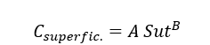 (23)
(23)
For Ctemp, it is known that the tests performed in the laboratory are performed in a controlled temperature environment. According to Shigley (2016), the inflection of the S-N curve tends to disappear at high temperature values. It is suggested that the following values be adopted: Up to 450°C the value of the correction factor must be 1.00. For temperature values between 450°C and 550°C, consider Equation 24.
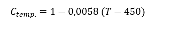 (24)
(24)
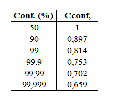
When it comes to reliability, the values obtained in tests refer to average estimates for several tests, where the deviation does not exceed 8%. Therefore, it is necessary to adopt a reliability factor according to Table 4.
Table 4: Reliability correction factor
It is also worth mentioning that the environment can significantly affect the fatigue strength of the part. Different results are found for tests with vacuum environment, atmospheric air and salt water environment.
Costa (2010), verified through experimentation, raising S-N curves of metallic materials, that in fact there is an uncertainty for the realization of a fatigue curve, which combined with all the variables already mentioned, together with the variations in the measurement methods and even in the machines to be used for the test, they make the engineer consider values that are often overestimated for the calculation of fatigue life.
According to Shigley (2016), the equations developed are related to the characteristics of the materials in a high cycle region, greater than. Norton (2004) mentions that with low-cycle information, it is possible to determine the S-N curve of the material. This data being (Sm), mean material resistance at cycles, as shown in Figure 6.
Figure 6: Estimated S-N curve
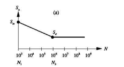
In the presence of normal force, the quoted average stress is equal to 75% of the ultimate resistance stress (Sut). The equation of the line passing through Sm and Se can be determined by Equation 25.
 (25)
(25)
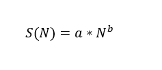
Where S(N) is the fatigue strength for an N number of cycles, a and b are constants defined according to boundary conditions.
The coefficients a and b are defined, respectively, by Equations 26 and 27.
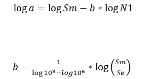 (26)
(26)
(27)
With this didactic, it is possible to analytically estimate the number of cycles that the shaft must support and the safety factor for fatigue resistance. This provides a starting point for numerical analyses.
According to Silva et al, the Finite Element Method (FEM) consists of a solution of differential equations by integration, applied on a set in smaller, discretized parts. The idea of separating the study domain into several smaller parts solves a problem regarding the difficulty of selecting interpolation functions that describe the behavior of the variables over the entire set.
For Silva (2016), it is possible to obtain, through the numerical use of the Ansys software, relative errors of 0.4%, comparing analytical voltage values in power transmission axes.
Gujaran and Gholap (2014) obtained less approximate results. Also through Ansys software, but for a more complex problem of fatigue in a shaft model with abrupt notches that resulted in an error of about 28%, when comparing numerical and analytical results. As for Engel and Al-Maeeni (2017), the relative error was about 7% in the maximum principal stress of a rotating axis of a bending machine.
For Dejan (2012), although calculations and numerical simulations pointed to a life of 2,000,000 hours of a hydroelectric turbine drive shaft, it failed with just over 1,000,000 hours at a known point of concentration. The hypothesis raised is that this point in constant tension becomes more susceptible to corrosion.
It is noticed that the complexity of the problem can directly influence the assertiveness rate of the calculations applied in this research.
RESULTS
All the calculations performed in this work were based on the technical engineering literature. The data obtained analytically follow protocols for dimensioning in terms of fatigue strength, aiming to find the failure region of the exhaust shaft under analysis.
Knowing the operating characteristics of this centrifugal fan, the flow being 300,798 m³/h, static pressure of 290 mmCA and the diameter of the rotor 2.95 m; an axial force of 19,638N is estimated, adding the results of equations 1 and 2.
Assuming that the fan works at most 10% outside the optimal operating point, through equations 3 and 4, the radial force generated by the change in air flow direction is estimated, which is around 35 N.
Considering that no rotating body obtains 100% balance, as indicated in the literature, in this case the highest possible value of residual unbalance mass was adopted. Knowing that the shaft rotation is 590 RPM and the balance quality grade adopted for this type of machine is G6.3; a specific unbalance of 100 g.mm/kg is estimated through the graph of Figure 3. Considering the worst case and applying this mass to the outer diameter of the rotor in Equations 5 and 6, the result for unbalance force is 878 N.
The pulleys measure 340 mm and 686 mm and the distance between centers is approximately 3850 mm. Considering a friction coefficient of 0.25 and the engine torque of 2,403 N.m applied to Formulas 7, 8, 9, 10 and 11, there is a tensioning force of the belts on the axle of 38,000 N.
Once the motor power and shaft rotation are known, the literature indicates that the nominal operating torque follows Equation 12, resulting in 4,855 N.m.
It is possible to adopt as power for this formula, the value that is consumed by the fan operation, calculated by multiplying flow in m³/s by static pressure in Pa; for this second hypothesis, the nominal torque would be 4,272 N.m.
From these technical memorial data, the shear force and bending moment graphs can be assembled, as shown in Figure 8.
Based on this and on the model notches, three points were selected to calculate the stresses, as shown in Figure 7; P1, P2 and P3.
Figure 7: Axis calculation points
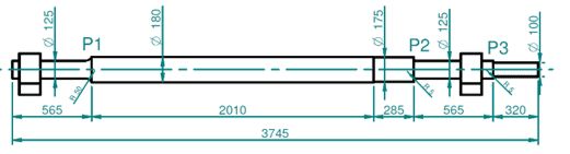
Figure 8: Shear force and bending moment graph
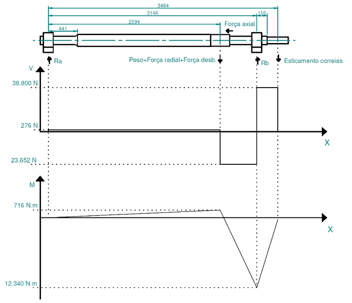
The bending moments generated on the axis at the points of analysis are the following: M1 which is 121.4 N.m; M2 is 2,655 N.m and M3 6,984 N.m.
For each of the selected points, it is necessary to calculate the geometric stress concentrator kt, according to the type of load which is imposed, Equation 13, Table 1.
Afterwards, through the Neuber constant for Steels, Table 2 and Equation 14, each of the notch sensitivity values is estimated and applied to Equation 15, which indicates the stress concentration values for dynamic stresses kf.
The shaft is fixed in the axial direction only at the point of Ra, so it is estimated that the axial force generates tensions only at Point 1, considering that it is applied to the shaft in the part with a diameter of 175 mm, from right to left, see Figure 8.
At point 1, the voltage values found, following Equations 16, 17 and 18, already applying increases by their respective kf, were:
![]()
For Point 2, which does not have tension by axial force, the same calculations indicated tensions of the following magnitudes, also already applied Kf factors:
![]()
Moving on to Point 3, the values found for the bending and torsional moments: ![]()
All the calculation hypotheses adopted took into account the worst possible boundary conditions, conditioning the results to the worst case within the tolerances that govern the operation of a fan and dimensioning of an axis.
With these data, we can determine the stress state at the mentioned points by estimating the Von Mises Stresses and using them to calibrate the numerical model. Von Mises values for points P1, P2 and P3 were respectively 24.40 Mpa, 47.50 Mpa and 141.90 Mpa.
The calculation of the number of cycles will take into account the maximum main voltage values, which through Equation 20, finds values of 15.43 Mpa; 49.85 Mpa and 135.85 Mpa for Points 1, 2 and 3.
Since the material shaft is SAE 1045, for the calculation of the fatigue strength limit it was necessary to consider E=206.8 Gpa, Sut= 690 Mpa and Sy= 580 Mpa. The fatigue analysis point will be P3.
To apply Equation 21, some considerations were made. Cload for Normal force presence is 0.7. CSize for a 100 mm shaft is 0.7606. For a machined surface, Csurf is 0.958. The design temperature of 160°C has no influence on the model. For 99.99% reliability, Cconf is 0.702.
Under these conditions, the axle fatigue strength limit is 124.40 Mpa. For a model with normal strength, the average strength was 517.5 Mpa. Thus, the estimated S-N curve for this axis is represented in Figure 9.
Figure 9: Estimated S-N curve
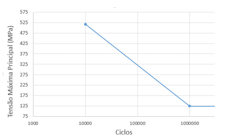
Knowing that the maximum principal stress resulted in 135.85 Mpa at point three and applying Equations 25, 26 and 27, it is analytically estimated that the shaft supports 653,978 cycles.
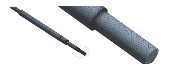
The numerical approximation modeled using Ansys software was initiated with the discretization of the model with a mesh of about 160,000 second-order tetrahedral elements, 238,544 nodes, with a refinement rate of 1 at the notch points, as shown in Figure 10.
Figure 10: Drive Shaft Mesh
To arrive at a mesh of satisfactory quality without consuming excessive execution time and that, on the other hand, does not present distortions and singularity stresses, the convergence curve was calibrated based on the Von Mises voltage value, see Figure 11.
Figure 11: Convergence curve
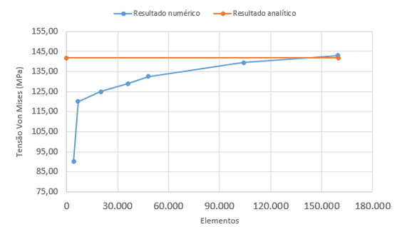
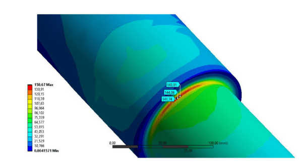
The structural static analysis resulted in stress values in the range of 144 Mpa, as shown in Figure 12, compared to the analytical 141.90 Mpa. A perfectly acceptable variation that shows good static resistance to failure, as the material used has a yield strength of 580 Mpa.
Figure 12: Von Mises Stress Point 3
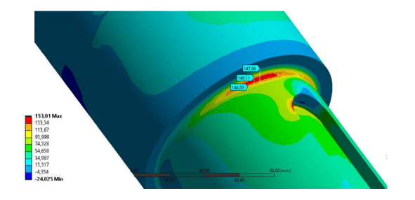
The axle fatigue life analysis took into account the maximum principal stress values, which numerically are in the range of 149 Mpa, against the analytical 135.85 Mpa. Figure 13 illustrates the P3 voltage concentration region.
Figure 13: Maximum main voltage
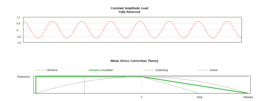
The fatigue life analysis execution module was carried out using the Ansys Transient structural, with the axis subjected to a completely reverse load and the Goodman Method, as shown in Figure 14.
Figure 14: Analysis execution mode
The stress-strain curve of the material used for fatigue life was from the Ansys database, for SAE 1045 Steel.
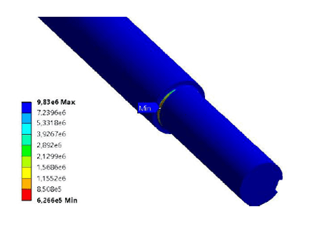
Spindle rotation as specified is 590 RPM, so each 1 second cycle equals 9,833 repetitions. The simulation demonstrated a life of 626,600 cycles for the critical region analyzed, as shown in Figure 15.
Figure 15: Number of Axis Life Cycles
Analyzing the durability of the part in hours, considering the work rotation of the axis and that for each turn is a cycle, the model would have a useful life of only 174 hours.
In the case of equipment that works 24 hours a day, the failure would occur in just one week.
The fact is that the axle fatigued and needed a replacement. There are no exact records of how long it took to fail, due to industrial secrecy, but the studies make clear the susceptibility of the part in the region of analysis.
All boundary conditions were measured at their upper limit, leading the results to show how the axis would behave under extreme conditions. The same showed that it would fail catastrophically in a short time for such parameters, but it is possible that the case under study has gone through milder requests until mechanical failure occurs.
Another point to be highlighted is the possibility of manufacturing failures, as highlighted by Di, Liang and Zhang (2016). A smaller than specified drive shaft stress concentrator radius can double the rated stress values during shaft operation and lead to premature and unforeseen failure by design.
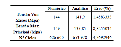
Evaluating the comparative parameters of the analyses, the consistency of the results can be seen, since the relative errors were low. Even the fatigue life results, the error between studies was about 4%, see Table 5.
Table 5: Relative error
Considering all the factors involved in the study and collection of data for dimensioning, calculation of requests and estimation of fatigue life, it was possible to contemplate the objective of parameterizing and obtaining this information in a practical way and based on calculations and computer simulations, supported by information from the piece previously manufactured and collapsed by working time; which demonstrates even more reliability in the method performed at work.
CONCLUSION
The drive shaft of a 400 hp exhaust fan failed due to fatigue during operation without having access to exact operating time information.
Aiming to estimate this time and the failure region, this research determined that in fact the failure was predictable even analytically. When comparing the analyses, the results were very good and maintained values of similar magnitudes.
The main objective of the study was to obtain parameters for the calculation of the exhaust shaft. This involves operating characteristics of flow machines and their nuances. Once the failure is known, the equation can be corroborated together with the simulation with the information to which we had access.
This is an important development when it comes to dimensioning in the flow machinery industry, it may be the basis for future studies and shaft dimensioning for future projects, or even testing changes to the design of this axis aiming at infinite life.
REFERENCES
ANDRESEN, P.; ANTOLOVICH, B. Fatigue and Fracture. ASM Handbook. 1997.
CALLISTER, William. Ciência e Engenharia de Materiais. 5. ed. Rio de Janeiro, RJ: Editora LTC, 2002. 589 p.
COSTA, Leandro Pereira. Avaliação da incerteza de medição no levantamento de curvas de fadiga S-N de materiais metálicos. 2010. Dissertação de Mestrado (Mestrado em Engenharia) – Universidade Federal do Rio Grande do Sul, [S. l.], 2010.
DU, Jinfeng; LIANG, Jun; ZHANG, Lei. Research on the failure of the induced draft fan’s shaft in a power boiler. Engineering Failure analysis, 2016.
ENGEL, B; AL-MAEENI, Sara Salma Hassan. Failure analysis and fatigue life estimation of a shaft of a rotary draw bending machine. International Journal of mechanical and mechatronics engineering, 2017.
GARCIA, A.; SPIM, J. A.; SANTOS, C. A.; Ensaios dos materiais. LTC – Livros técnicos e Científicos Editora Ltda, Rio de Janeiro – RJ, 2012.
GUJARAN, Sandeep; GHOLAP, Shivaji. Fatigue Analysis of Drive Shaft. International Journal Of Research In Aeronautical And Mechanical Engineering, [S. l.], p. 1-8, 10 out. 2014.
GUJAR, R. A.; BHASKAR, S. V. Shaft Design under Fatigue Loading By Using Modified Goodman Method. International Journal of Engineering Research and Applications, [S. l.], p. 1061-1066, 1 ago. 2013.
HENN, Érico Antônio Lopes. Máquinas de Fluido. 2. ed. Santa Maria, RS: Editora da UFSM, 2006. 476 p.
HIBBELER, R. L. Resistência dos materiais. 7. ed. São Paulo: Pearson Prentice Hall, 2009.
INTERNATIONAL ORGANIZATION FOR STANDARDIZATION. ISO 1940:2003. Vibração Mecânica – Requisitos de qualidade de balanceamento para rotores rígidos, [S. l.], 15 ago. 2003.
JORGENSEN, R. Fan Engineering. 9 ed. Buffalo, New York: Howden Buffalo, Inc.: 1999.
MOMČILOVIĆ, Dejan et al. Failure analysis of hydraulic turbine shaft. Engineering Failure Analysis, 2012.
NISHI, E. K. Apostila de balanceamento. Londrina: Nishi eletromecânica, 2006
NORTON, Robert L. Projeto de Máquinas: Uma abordagem integrada. 2. ed. Porto Alegre – RS: Editora Bookman, 2004. 905 p.
ROY, Ankita et al. Investigation of torsional failure of a centrifugal pump shaft. Engineering Failure analysis, Kalinganagar, India, 2020.
SCHIEL, Frederico; Introdução a resistência dos materiais. São Paulo, SP : Editora Harper & Row do Brasil., 1984. 395 p.
SHAHROOI, Shahram; ASAYESH, Masood. Numerical and experimental analysis for fatigue failure investigation on gas recirculation fan shaft. 9th International Conference on Fracture and Strenght of solids, Korea, 2013.
SHIGLEY, J. E. Elementos de máquina. 10. ed. Porto Alegre – RS: Editora AMGH, 2016. 1096 p.
SILVA, J. G.; SOEIRO, F. J.; TRIGUEIRO, G. S.; ROBERTO, A. R.; Análise Estrutural de Chassis de Veículos Pesados com Base no emprego do programa Ansys. Cobenge, Rio de Janeiro, 2001.
SILVA, F. A.; CHAVES, C. A.; GUIDI, E. S.; Análise de falha por fadiga em eixo de transmissão utilizando o método dos elementos finitos. Exacta – EP, São Paulo, v. 14, n. 2, p. 207-219,2016.
TREBUNA, F. et al. Identification of causes of radial fan failure. Engineering Failure Analysis, Kosice, Eslováquia, 2009
ZAMBRANO, O. A.; CORONADO, J. J; RODRIGUEZ, S. A. Failure analysis of a bridge crane shaft. Engineering Failure analysis, 2014.
[1] Specialist in Predictive Structural Engineering, Mechanical Engineer and Technician in Industrial Automation. ORCID: 0000-0003-4407-3351.
[2] Advisor. ORCID: 0000-0001-7965-1620.
Sent: May, 2022.
Approved: September, 2022.