ORIGINAL ARTICLE
PEREIRA, Sérgio Rodrigo Araújo [1], BRAGA, Eduardo de Magalhães [2]
PEREIRA, Sérgio Rodrigo Araújo. BRAGA, Eduardo de Magalhães. Influences of roughness levels on the results of chemical analysis by optical emission spectrometry. Revista Científica Multidisciplinar Núcleo do Conhecimento. Year 05, Ed. 03, Vol. 09, pp. 102-121. March 2020. ISSN: 2448-0959, Access Link: https://www.nucleodoconhecimento.com.br/engineering-mechanical-engineering/roughness-levels
SUMMARY
The present study aims to investigate the influences of roughness levels, after chemical analysis by optical emission spectrometry, in order to verify in which sanding step the chemical composition of the low alloy steel rail (THH 370-JISE E1120), closer to the original factory standard. The roughness of the sample surface was measured at various levels (post cut, #60, #120, #220 and polished) and subsequently chemical analysis was performed by optical emission spectrometry. The results showed that the sanding stage with mesh 120#, presented the lowest relative errors of chemical composition and one of the roughness parameters (Ra, Rq, Rz) more homogeneous among the other phases analyzed. The chemical composition of the test body, after successive sanding and spectrometer burning, oscillated differently by chemical element analyzed.
Keywords: Roughness, optical emission spectrometry, sanding, low alloy steel, Roughness Parameters.
1. Introduction
During the development of an engineering project, the properties of the materials should be considered to determine the efforts and requests involved. As an example, in the design of an automotive shaft are checked all the properties of the mechanical construction steel used, as well as the components that attach it. Thus, it is essential that materials that meet the specifications determined in the project are used during the production process. For this due control, standardized mechanical, physical and chemical testing procedures are performed for quality control or material verification (PAHL, 2005; ASHBY, 2011).
In steels the chemical composition has a high influence on its physical, mechanical and chemical properties. These alloys have base elements such as iron (Fe) and carbon (C) (up to 2.11%), in addition to other chemical elements that promote different properties to steels. For example, the addition of chromium (Cr) in the alloy increases mechanical resistance, hardening, resistance to abrasive wear and corrosion. The addition of tungsten (W) increases the hardness and reduces the thermal conductivity of the steel alloy. As in the example described, both chemical elements modify the properties of steels, i.e., the absence of essential elements or too much presence may affect the properties required in the projection of the product or component (CHIAVERINI, 2008).
To determine the chemical composition of steels, one of the methods used is optical emission spectrometry. The operating principle of this method/equipment is based on the measurement of the three basic physical quantities of light or electromagnetic wave: intensity (or amplitude), frequency and polarization (vibration angle) (SERWAY, 2011).
2. EXPERIMENTAL PROCEDURE
In order to obtain the results proposed in this study, experimental procedures were performed. The tests were carried out in the Laboratory of Characterization of Metallic Materials (LCMM) of UFPA (Federal University of Pará), which will be described in detail the procedures, materials and equipment used.
The rails used for chemical analysis are of the model THH 370 (JISE 1120) of Japanese manufacture, whose manufacturing process is through the reduction of iron ore in high ovens for the production of pig iron, later the material passes through the steel industry, lamination, heat treatment and alignment. Table 1 illustrates the chemical composition of the THH 370 rail.
Table 1 – Chemical composition of the THH 370 rail (JISE 1120)
| C | Si | Mn | P | S | Cr | Other |
| 0,79 | 0,17 | 0,99 | 0,030≤ | 0,020≤ | 0,16 | V:0.03 max |
Source: (JFE, 2014).
Table 1 identifies only the six main constituent elements of the chemical composition of the THH 370 rail, supplied by the manufacturer, which will be based on the proposed analysis.
To achieve different levels of roughness, the test body underwent a sanding process with different sandpaper particlesizes, as illustrated in table 2.
Table 2 – Identification of the different surface preparations used in the experiment.
| Identification | 1 | 2 | 3 | 4 | 5 |
| Granulometry | Post-cut | #60 | #120 | #220 | Polished |
Source: (Author).
After the sanding process with metallographic politriz (Model Fortec II), the test body was submitted to cleaning with isopropyl alcohol. Cleaning was performed to prevent the presence of contaminants in the analysis of chemical composition. Subsequently, the roughness of the test body was evaluated.
For roughness measurement, a portable rugosimeter Mitutoyo, surft Sj 210 model, adjusted to measure 5 sampling lengths (λs) of 2.5 μm generating a cut off length of 0.8 mm was used. The measurements were performed in 2 different positions, fulfilling the transverse direction (90º) of the grooves of the test body, being considered the average of the values obtained for the analysis of the results. In addition to the profile, the evaluation of the roughness of the profile of the test body was performed in the parameters Ra, Rq and Rz (WHITEHOUSE, 2003). Figures 1 and 2 illustrate the test body and the rugosimeter apparatus respectively.
Figure 1 – Test body analyzed
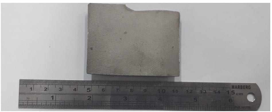
Figure 2 – Mitutoyo Model Surft SJ 210 Portable Rugosimeter
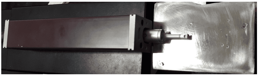
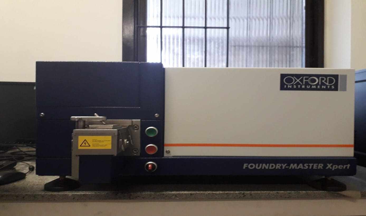
For the chemical composition assay, the oxford manufacturer’s optical emission spectrometer, foundry master Xpert model, was used. It should be noted that before this experiment, the proper procedures were performed according to the manufacturer’s guidelines.
Initially to avoid any type of contamination and inaccuracy in the results, the instrument was purified with argon gas, compressed under pressure of 3.0 bar, 24 hours before the start of the analyses, with the aid of a vacuum pump.
Figure 3 – Vacuum pump used in the purification of the spectrometer

The electrode holder, as well as the electrode used for the spark (in this case, Fe electrode), were cleaned with a brush. Soon after, it was installed on the stand, with the aid of an Allen key. The spacing between the electrode tip and the sample surface was adjusted to 3.2 mm using a spacer, according to the manufacturer’s manual guidelines.
For the processing of the data, a computer was turned on and the Waslab software, properly activated. The selected analytical program was the Fe_100, ideal for analysis of low alloy steels. The sample was placed on the spark holder with the side to be analyzed down.
Figure 4 – Optical Emission Spectrometer
For each surface preparation (samples 1 to 5), the number of burns in the spectrometer was repeated 10 times, allowing the comparison of samples by analysis of variance using a confidence interval of 99.7%.
Therefore, each test consisted of the preparation of the surface of the test body (calibration standard), the sanding procedures, the roughness measurement and the chemical composition assay. For each new preparation, the proper procedures were repeated.
3. RESULTS AND DISCUSSIONS
3.1 ROUGHNESS ANALYSIS
3.1.1 ROUGHNESS – STEP 1
According to the generated surfaces and the predefined steps, roughness analyses are arranged, these being measured in two directions: one longitudinal and the other in the transverse direction.
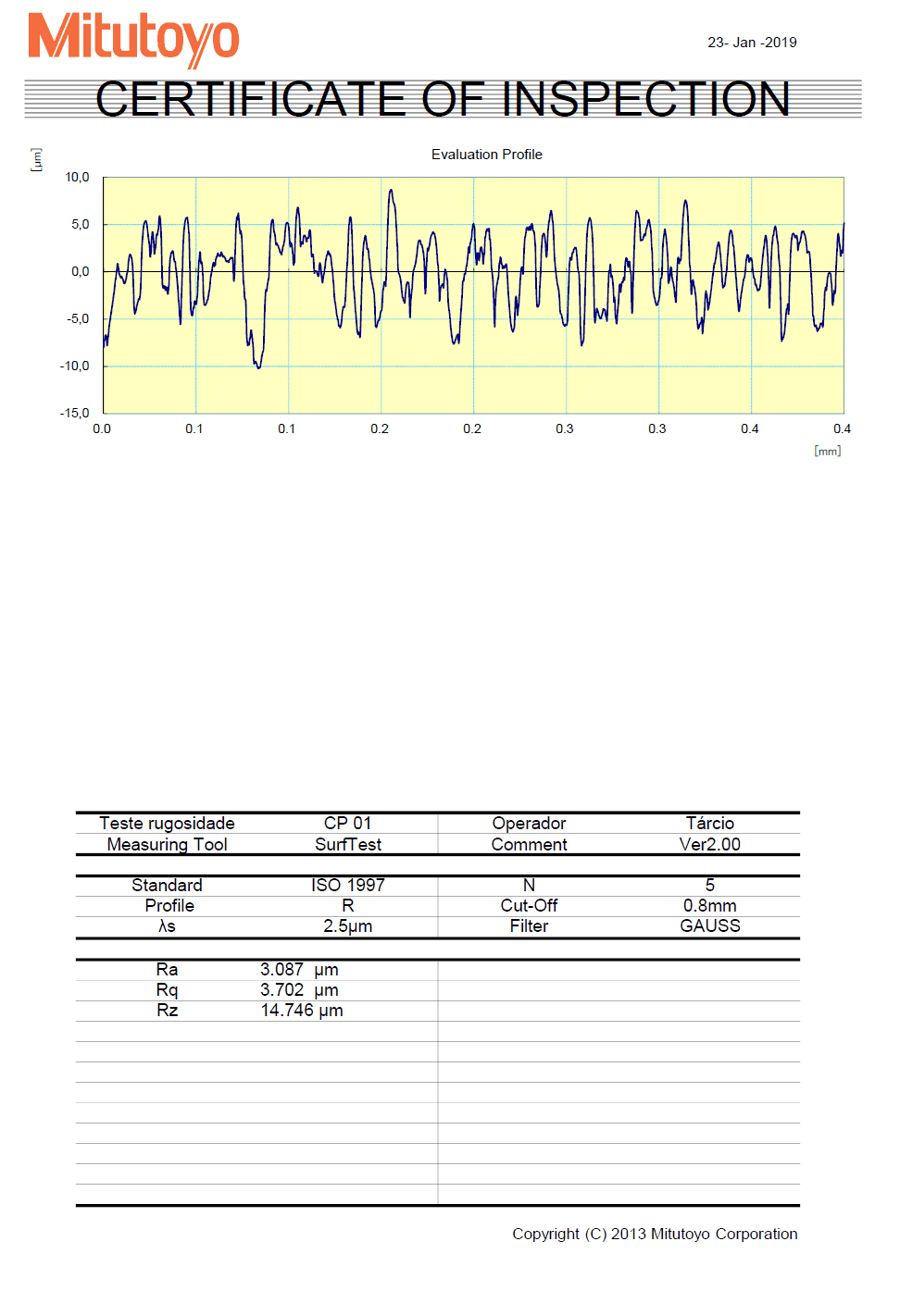
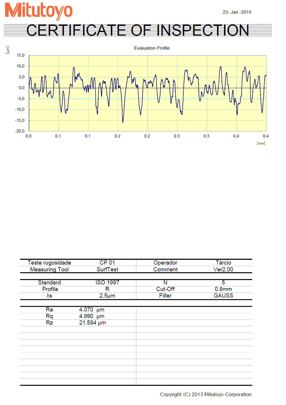
Below are listed the averageroughness found in the test body after successive sanding. Table 3 shows the mean roughness in the longitudinal and transverse directions in the test body after cutting. It is necessary to emphasize that the cut in the test body was made by electroerosion.
Table 3 – Longitudinal and transverse roughness measurement (post-cut)
| Parameter | Longitudinal | Cross |
| Ra | 3,087µm | 4,070 µm |
| Rq | 3,702 µm | 4,990 µm |
| Rz | 14,746 µm | 21,584 µm |
Source: (Author).
As we can observe, in this first result, the Values Ra and Rq, are – they are very approximate, while there is a large discrepancy in relation to the value obtained in Rz, both in the longitudinal and in the transverse, which is normal because Rz is a parameter that indicates the height of the maximum and minimum points of the profile, and the difference between the values in the crossis is noisily more marked. This is due to the form of sanding, in this case, the transverse direction predominated.
3.1.2 ROUGHNESS – STEP 2
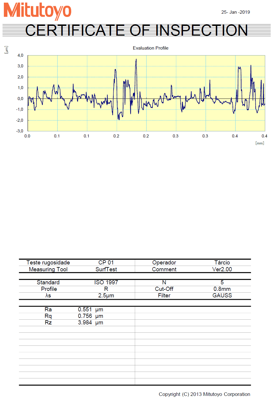
Subsequently, the surface of the test body was submitted to its first stage of sanding with mesh #60, obtaining the values described in table 5. There is a sharp decrease in the roughness values in relation to the previous stage in both directions of the measurement, however, there is a certain difference favorable to the transverse direction.
Table 4 – Longitudinal and Transverse Roughness Measurements (#60)
| Parameter | Longitudinal | Cross |
| Ra | 0,551 µm | 1,291 µm |
| Rq | 0,756 µm | 1,705 µm |
| Rz | 3,984 µm | 9,709 µm |
Source: (Author).
3.1.3 ROUGHNESS – STEP 3
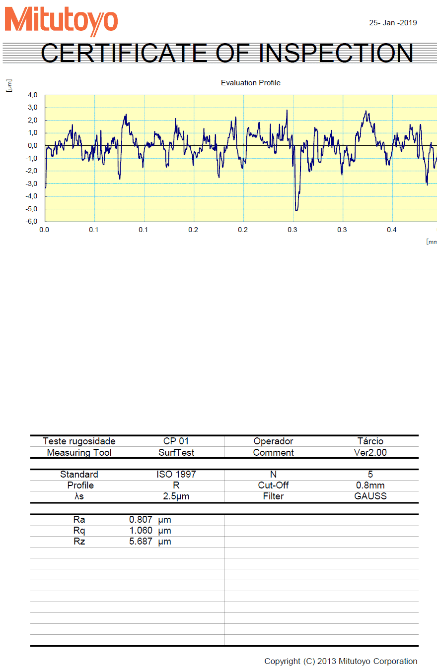
The next step of sanding the surface of the test body was performed with mesh sandpaper #120, obeying the same parameters as the previous sanding. The measurement of roughness of the longitudinal and transverse senses reached homogeneous values. The following values were obtained in Table 5.
Table 5 – Longitudinal and Transverse Roughness Measurements (#120)
| Parameter | Longitudinal | Cross |
| Ra | 0,807 µm | 0,901 µm |
| Rq | 1,060 µm | 1,184 µm |
| Rz | 5,687 µm | 7,708 µm |
Source: (Author).
3.1.4 ROUGHNESS – STEP 4
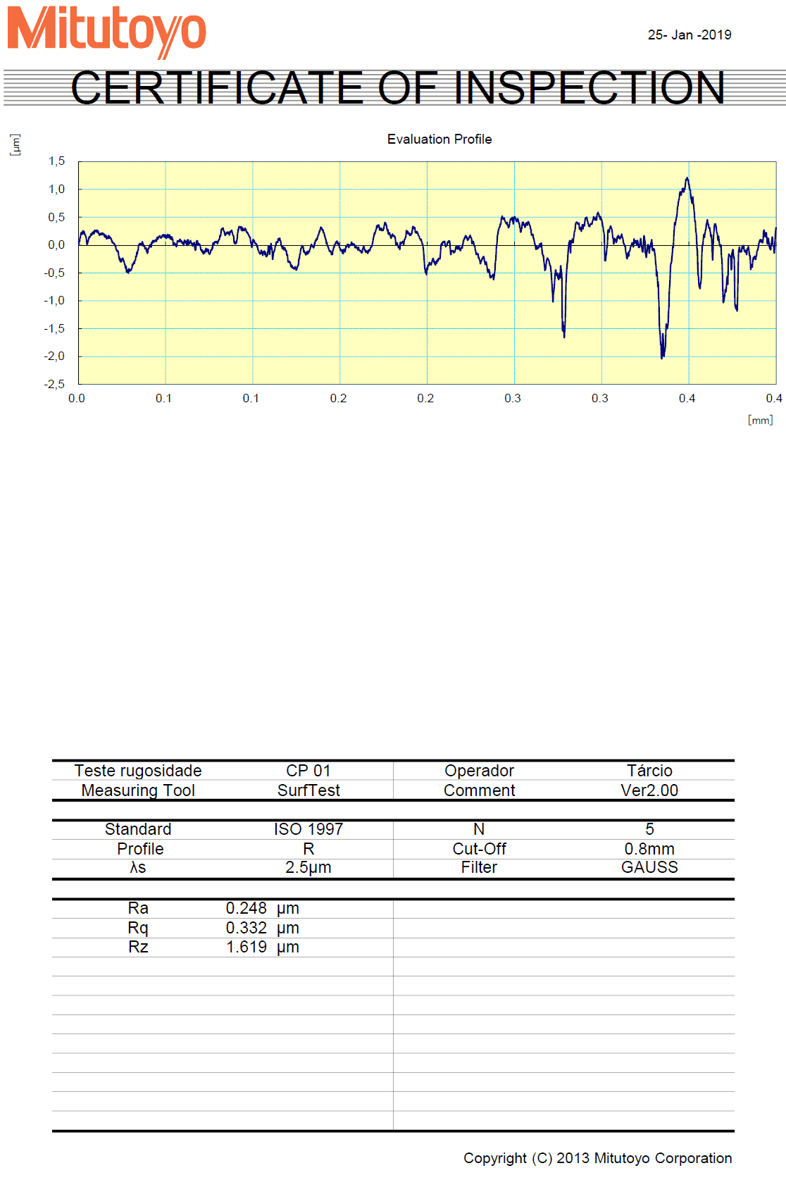
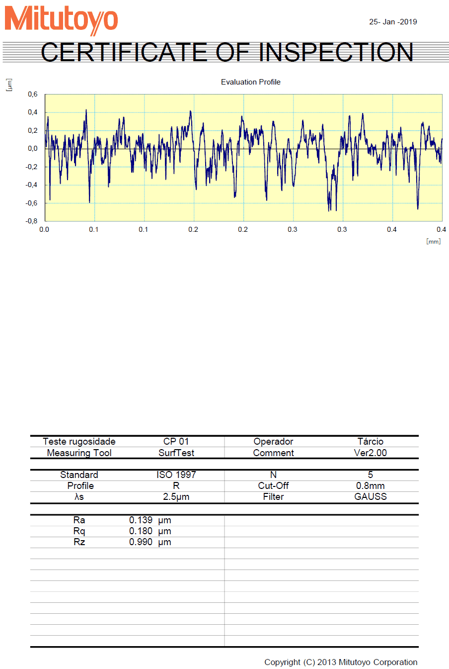
At this stage, the surface of the test body was sanded with mesh sandpaper #220, which is observed, that the roughness values in the longitudinal direction became higher than in the transverse direction for the first time in this experiment, generating the following values attached in table 6.
Table 6 – Longitudinal and Transverse Roughness Measurements (#220)
| Parameter | Longitudinal | Cross |
| Ra | 0,248 µm | 0,139 µm |
| Rq | 0,332 µm | 0,180 µm |
| Rz | 1,619 µm | 0,990 µm |
Source: (Author).
3.1.5 ROUGHNESS – STEP 5
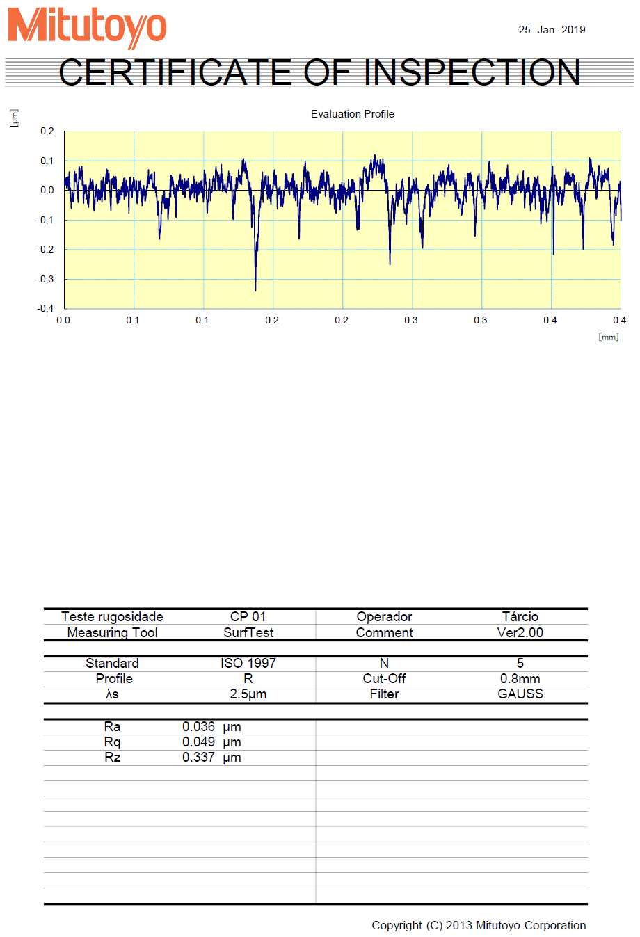
In this last stage, the test body was submitted to the polishing process being sanded with different types of sandpaper (#40, #60, #120, #220, #600), and properly cleaned for removal of any metal remnants. Roughness results were obtained, homogeneous in both directions, and in the longitudinal sense the values prevailed slightly higher. The measurements are at the table 7.
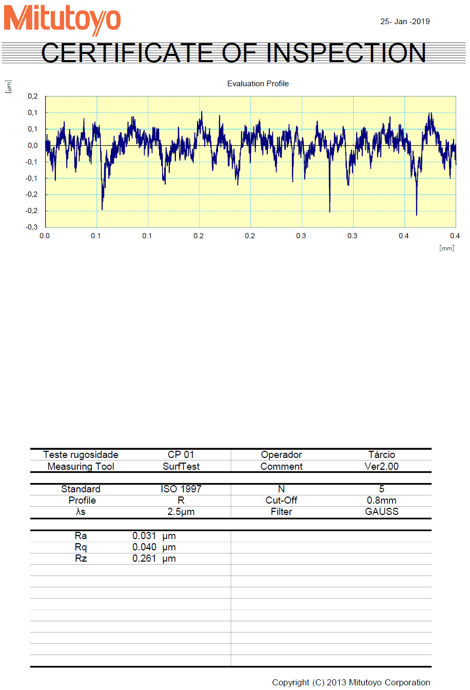
Table 7 – Longitudinal and Transverse Roughness Measurements (Sup. Polished).
| Parameter | Longitudinal | Cross |
| Ra | 0,036 µm | 0,031 µm |
| Rq | 0,049 µm | 0,040 µm |
| Rz | 0,337 µm | 0,261 µm |
Source: (Author).
3.2 CHEMICAL ANALYSIS BY (EEO)
After the sanding and roughness measurement phase, the chemical analysis was performed by optical emission spectrometry of the test body. For each sandpaper particle applied to the surface of the workpiece, its chemical composition was measured, and with the data obtained, a relative error analysis was performed to verify which roughness level closest to the standard chemical composition of the rail in question. Table 8 illustrates the values obtained in all sanding steps and their absolute standard deviation, respectively.
Table 8 – Chemical composition of the surface of the test body and standard deviation.
| Mesh# | C | Si | Mn | P | S | Cr |
| Polished | 0,858 ± 0,015 | 0,250 ± 0,0108 | 1,19 ± 0,009 | 0,0100 ± 0,0008 | 0,001 ± 0,0011 | 0,186 ± 0,0020 |
| 220 | 0,841 ± 0,017 | 0,260± 0,0115 | 1,17 ± 0,015 | 0,0105 ± 0,0002 | 0,001 ± 0,0010 | 0,186 ± 0,0027 |
| 120 | 0,821 ± 0,013 | 0,243± 0,0076 | 1,20 ± 0,017 | 0,0131 ± 0,0001 | 0,002 ± 0,0012 | 0,190 ± 0,0026 |
| 60 | 0,841 ± 0,024 | 0,255± 0,0114 | 1,19 ± 0,012 | 0,0117 ± 0,0001 | 0,001 ± 0,0013 | 0,187 ± 0,0017 |
| Post-cut | 0,916 ± 0,048 | 0,247 ± 0,0130 | 1,20 ± 0,001 | 0,0106 ± 0,0001 | 0,001 ± 0,0000 | 0,190 ± 0,0022 |
Source: (Author).
3.3 RELATIVE ERROR OF CHEMICAL ELEMENTS
According to the data described, the S had the highest relative error rate, indicating that its values are relatively less close to the value of the standard, and in turn the Cr achieved error rates between 0.1 and 1.5%. Table 9 describes the percentage values of relative error, as we can see.
Table 9 – Relative error by chemical element in (%).
| C | Si | Mn | P | S | Cr | |
| Post-cut | 16 | 45 | 22 | 64 | 95 | 0,1 |
| # 60 | 6,4 | 53 | 20 | 61 | 93,5 | 1,5 |
| # 120 | 3,9 | 41 | 21 | 56 | 90 | 0,1 |
| # 220 | 6,4 | 53 | 18 | 50 | 95 | 0,4 |
| Polished | 47 | 47 | 20 | 66 | 94,5 | 0,4 |
Source: (Author).
It is noted that in the sanding stages #120 and #220, there is greater homogeneity in the results, illustrating the two lowest series of relative error rates in relation to the other stages of sanding.
4. CONCLUSION
Based on the data obtained, it was observed that the values found in the parameters Ra, Rq and Rz in the 120# mesh had one of the most homogeneous behaviors among the others, and with lower rate of relative error of chemical composition of the low alloy steel rail. The Rz parameter was the one that provided the highest values, which was expected, due to the same being the mean between the minimum and maximum roughness points of the midline, while the parameters Ra and Rq, had homogeneous behavior, with timid oscillation during the steps. From the sanding with mesh 220# the roughness values in the longitudinal direction became higher than in the transverse direction, however, all parameters after this stage presented roughness values very approximate.
The sanding with mesh 120# presented the lowest relative error in 4/6 of the analyzed elements, which were: C, Si, S and Cr. It is important to highlight that in the chemical elements P and Mn, their relative error was the second lowest.
In the stages where the roughness parameters showed greater homogeneity, both in the transverse and longitudinal sense, the relative error rates were the lowest.
Therefore, 120# mesh sanding proved to be a fast and inexpensive surface treatment solution, since, based on the acquired data, its action in low alloy steel approached, in terms of chemical composition, to the levels established by the rail manufacturer THH 370 (JISE E1120).
REFERENCES
ASHBY, Michael F. Materials selection in mechanical design. 4th ed. Amsterdam: Elsevier, 2011. 646 p. 17
CHIAVERINI, Vicente. Aços e ferros fundidos: características gerais, tratamentos térmicos, principais tipos. 7. ed. ampl. e rev. São Paulo: Associação Brasileira de Metalurgia e Materiais, 2008. 599 p.
JFE-STEELCO, 2014. http://www.jfe-steel.co.jp/en/release/2014.html. Acessado em: 17/02/2019.
PAHL, Gerhard. Projeto na engenharia: fundamentos do desenvolvimento eficaz de produtos, métodos e aplicações. São Paulo: Edgard Blücher, 2005. 412 p.
SERWAY, Raymond A; JEWETT Jr, John W. Física para cientistas e engenheiros: eletricidade e magnetismo. São Paulo: Cengage Learning, 2011.
WHITEHOUSE, D. J. Handbook of surface and nanometrology. 1 ed. ed. Bristol: IPP Publisher, 2003. 1128 p.
ANNEX
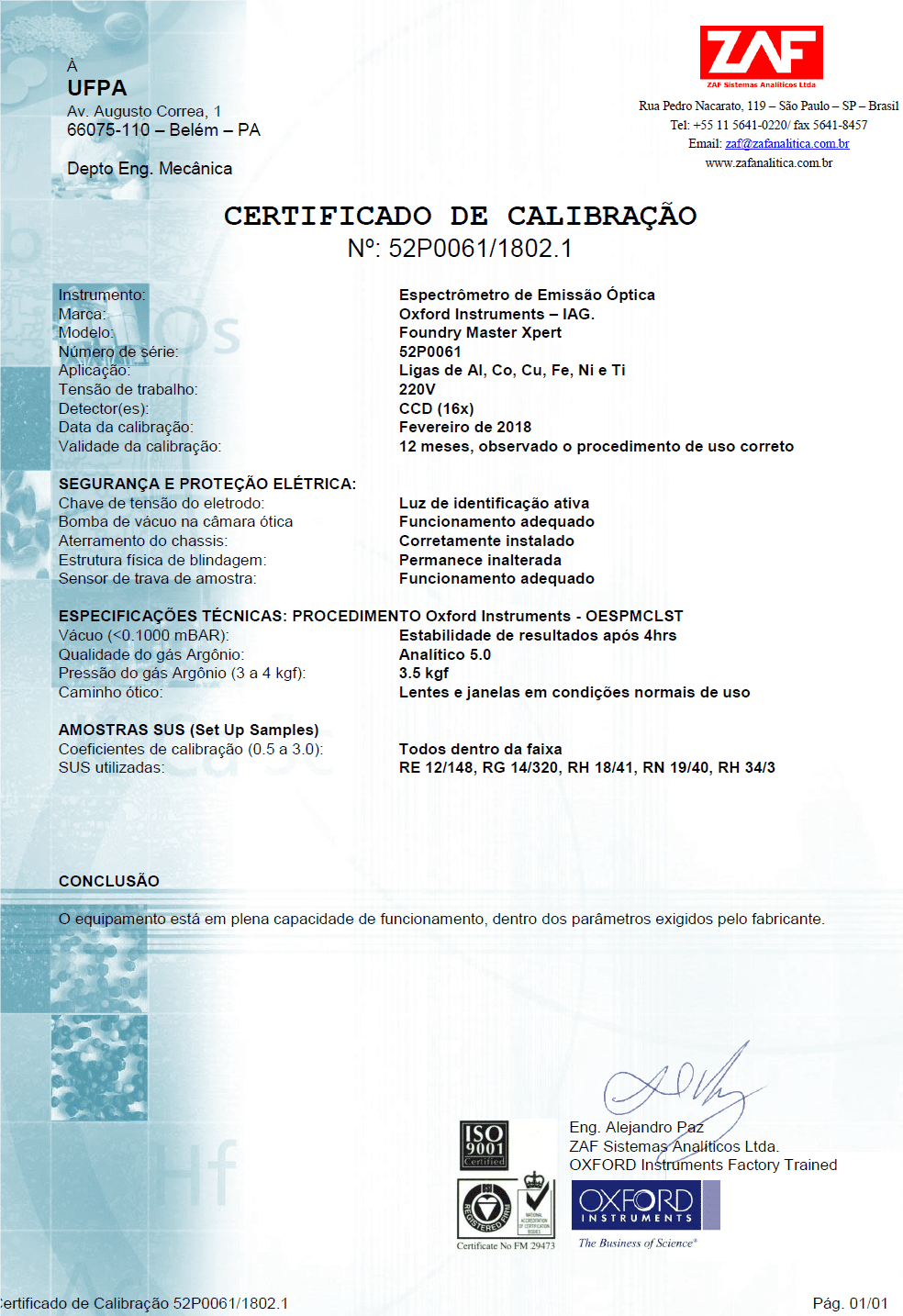
ANNEX I – Spectrometer Calibration Certificate
ANNEX II – Roughness Analysis Certificate (Post cut – longitudinal)
ANNEX III – Roughness Analysis Certificate (Post cut – transversal)
ANNEX IV – Roughness Analysis Certificate (Mesh 60 # – longitudinal)
ANNEX V – Roughness Analysis Certificate (Mesh 60 # – transversal)
![]()
ANNEX VI – Roughness Analysis Certificate (Mesh 120 # – longitudinal)
ANNEX VII – Roughness Analysis Certificate (Mesh 120 # – transversal)
![]()
ANNEX VIII – Roughness Analysis Certificate (Mesh 220 # -longitudinal)
ANNEX IX – Roughness Analysis Certificate (Mesh 220 # – transversal)
ANNEX X – Certificate of Roughness Analysis (polished-longitudinal)
ANNEX XI – Roughness Analysis Certificate (polished-transversal)
[1] Mechanical Engineering Student (UFPA).
[2] PhD in Mechanical Engineering. Master’s degree in Mechanical Engineering. Degree in Mechanical Engineering.
Submitted: October, 2019.
Approved: March, 2020.