REVIEW ARTICLE
VICTORINO, Samuel Carlos [1]
VICTORINO, Samuel Carlos. Another approach on elaborating frequency tables using GAUSS´s normal distribution theory. Revista Científica Multidisciplinar Núcleo do Conhecimento. Year 06, Ed. 03, Vol. 07, pp. 139-154. March 2021. ISSN:2448-0959, Access link: https://www.nucleodoconhecimento.com.br/agronomy-en/frequency-tables, DOI: 10.32749/nucleodoconhecimento.com.br/agronomy-en/frequency-tables
ABSTRACT
The correct organization of data is of extreme importance for the analysis in the process of statistical inference, aiming at the elaboration of valid conclusions and generic recommendations on a certain subject under study. The specialized scientific literature describes several procedures for the organization of data in frequency distribution tables. However, it is not often that inaccuracies are made in the use of data organization tools. These inaccuracies have resulted in distorted analyzes and incongruous conclusions. This paper presents a critical analysis of the methods and procedures of data organization described in the literature, specifically the distribution of data in frequency distribution tables and proposes a different approach in the elaboration of class frequency distribution tables. For all variables with predefined categories, these and their respective reference values serve as the body of the table. For the variables that do not have pre-defined categories, the use of Gauss’s normal distribution theory as a criterion for categorization is proposed and justified. The categories generated serve as a table body. It is concluded that the frequency distribution tables can be distinguished into two types, that is, frequency distribution tables of predefined classes or categories and tables of frequency distribution of classes or categories to be defined, thus suggesting their adoption as concept.
Keywords: Normal distribution, Simple frequency distribution table, Frequency distribution table of predefined classes, Frequency distribution table of classes to be defined.
1. INTRODUCTION
Statistics, as a science, is summarized in a set of methods and procedures that allow the collection, organization and presentation of data for their analysis, in order to obtain valid conclusions and the elaboration of generic recommendations on a given population being studied.
Statistics finds application in the most diverse areas of knowledge such as economics, psychology, sociology, agriculture and health, helping in the decision-making process based on data analysis. In order for statistics to fulfill this role, it is imperative that the methods and procedures are properly applied. Data collection involves the correct application of sampling methods which culminate in the selection of representative samples and ensure the validity of the data and, at the same time, the validity of the studies; the organization and presentation of data aims the simplification and compression of data into frequency distribution tables, whether they are single frequency tables or class frequency tables. Data summarized in tables are generally, and where appropriate, visualized in graphs, diagrams and other statistical tools. Their correct organization is of extreme importance for data analysis in the process of statistical inference.
The specialized scientific literature describes a wide range of procedures for data organization in frequency distribution tables. It has been found that inaccuracies in the use of data organization tools are often committed, resulting in distorted interpretation and incongruent conclusions. This article aims to present a critical analysis of the methods and procedures of data organization described in the literature, specifically the data distribution in frequency tables and proposes a different approach in the elaboration of frequency distribution tables.
2 . THEORETICAL FRAMEWORK ON FREQUENCY DISTRIBUTION TABLES
The statistic is divided into two main groups: descriptive statistics and inferential statistics.
Descriptive Statistics is the part that deals with the description, classification, organization and presentation of the data of a variable. It allows summarizing data and helps describing the attributes of a given data group or a population by means of the calculation of descriptive measures such as the mean and the standard deviation. The tabular and graphic descriptive techniques used with the support of the graphical capabilities of modern computers and the various software available make this type of summary more feasible and more understandable.
Inferential statistics, on the other hand, is responsible for analyzing data in order to obtain valid conclusions and the elaboration of generic recommendations about the population being studied.
2.1 TABULAR AND GRAPHIC DESCRIPTIVE TECHNIQUES
The raw data of a variable obtained in a sampling process do not allow the visualization of any characteristic of the sample and much less of the population under study. Therefore, tables and graphs are essential statistical resources in data processing.
Tables allow to summarize and compact a large amount of information providing a clear analysis to the researcher. Graphs are table’s complement that have the function of transmitting a visual idea of the data´s behavior. There is a wide variety of graphs, among them, line graphs, bar graphs, area graphs and pie charts as the most common. As for the frequency distribution tables, the following types are fundamentally different:
1 – Single frequency distribution table
2 – Class frequency distribution table
A single frequency distribution table contains two main columns. In the first column each collected value is inserted sequentially, once and in ascending order. In the second column in the line corresponding to each observed value is inserted the number of times that these values are repeated in the data set, which correspond to the respective absolute frequency.
The class frequency distribution table also contains two columns, the first for the class intervals of the variable and the second for the number of individuals belonging to each class, that is, the absolute frequency of the class.
Single frequency distribution tables have the major disadvantage of being too long, due to the fact that all sampled values have to be listed and, above all, do not allow the reading of data characteristics. These type of tables are totally inappropriate when the purpose is to summarize large amounts of data. For these cases, class frequency distribution tables are more suitable, as they compact large amounts of data into a few classes and link the quantitative attributes of the variable to the actual meaning of the characteristics of the variable.
The fundamental aspect in the elaboration of distribution tables of class frequencies is the determination of the number of classes, in which the data will be framed. For this purpose, several criteria for determining the number of classes are described in the literature, most of which are strictly mathematical based.
Milton and Tsokos (1991) indicate the use of the following formulas to determine the number of classes:
1 – Number of classes = 5 x lg n where n is the sample size
2 – Number of classes =![]()
Beiguelman (2002) indicates that the number of classes is between 8 and 20, depending on data. For Dawson and Trapp (2003) 6 and 14 classes are adequate to provide sufficient information without excessive detail. Triola and Triola (2006) recommend that the number of classes should be between 5 and 20, while Kuzma and Bohnenblust (2001) consider that the number of classes should be 5 to 15. Reis (2005) states that the number of classes should be between 4 and 14 and also suggests the use of one of the following solutions:
1 – Number of classes equal 5 for samples with size less than 25 and number of classes = ![]() for samples with a size equal or greater than 25.
for samples with a size equal or greater than 25.
2 – Use the Sturges formula: number of classes = 1 + 3,22 log n
The aforementioned shows the variety of criteria described within the literature for the construction of frequency distribution tables. However, these criteria have a common disadvantage that makes them unsuitable as a basis for determining the number of classes of data for certain variables, such as variables in the field of biology and health sciences, economics, industry, among others, which have pre-defined categories, that are, standardized categories. Some of these variables are described below and the respective reference values of the pre-defined categories are indicated.In the field of biology:
Example1: Reference values of total cholesterol in humans Table 1: Categories and reference values of total cholesterol in humans.
| Total Cholesterol | Category |
| < 200 mg/dl | Desirable or Normal |
| 200 – 239 mg/dl | Border |
| ≥ 240 mg/dl | High |
Source: Third Report of the National Cholesterol Education Program (NCEP) Expert Panel on detection, evaluation, and treatment of high blood cholesterol in adults (Adult Treatment Panel III). Final report. Circulation, 2002, 106:3143–3421
Example 2: Reference values for body mass index (BMI).
The BMI helps to define the obesity degree of a person according to the World Health Organization. By calculating and interpreting the BMI it is possible to know if a person is above or below the weight parameters recommended for their physical structure. To calculate the BMI, the weight measured in kg is divided by the height squared (BMI = kg / m2).
Table 2: Categories and reference values of Body Mass Index
| Category | BMI (kg/m2 ) |
| Underweight | < 18,5 |
| Normal (healthy weight) | 18,5 – 24,9 |
| Pre-obese | 25,0 – 29,9 |
| Obese class I | 30,0 – 34,9 |
| Obese class II | 35,0 – 39,9 |
| Obese class III | ≥ 40,0 |
Source: World Health Organization. Obesity (1998): Preventing and managing the global epidemic: report of a WHO Consultation on Obesity, Geneva, 3–5 June 1997. Geneva (CH): World Health Organization; 1998. http://whqlibdoc.who.int/hq/1998/WHO_NUT_NCD_98.1_(p1-158).pdf.
Example 3 – Classification of arterial hypertension. Table 3: Classification of arterial hypertension
| Classification of blood pressure | Sistolic blood pressure (mmHg) | Diastolic blood pressure (mmHg) |
| Normal | < 120 | < 80 |
| Pre-hypertension | 120 – 139 | 80 – 89 |
| Stage 1 (grade I) hypertension | 140 – 159 | 90 – 99 |
| Stage 2 (grade II) hypertension | ³ 160 | ³ 100 |
Source: The seventh report of the Joint National Committee on prevention, detection, evaluation, and treatment of high blood pressure. JAMA 2003; 289: 2560-72. Cited for PEDROSA and DRAGER (2010).
Example 4: Uric acid results from the metabolism of purines, major structural elements of DNA and RNA, much of it from food. Excessive consumption of meat or alcohol can raise levels of uric acid in blood.
Reference values are in general 40 a 60 mg/L for men, 30 a 50 mg/L for women and 25 a 40 mg/L for children (CAQUET, 2011).
In the field of economics:
Example 5: The Human Development Index (HDI) is a statistical data created by the United Nations Development Program (UNDP) to counter the purely economic data used to measure country wealth and to analyze development by including other factors.
For this variable the following categories are standardized under which countries are divided based on their respective HDI:
Low HDI: brings together all countries with HDI below 0.500.
Average HDI: countries with HDI between 0.500 and 0.799.
High HDI: countries with HDI between 0,800 and 0,899.
Very high HDI: countries whose HDI is equal to or above 0.900.
Source: PENA, Rodolfo F. Alves. “Como é feito o cálculo do IDH?”; Brasil Escola. Available on: https://brasilescola.uol.com.br/geografia/desenvolvimento-humano.htm. Retrieved on March 25, 2020.
The examples cited above show that the criteria with mathematical basis are not suitable for all situations. In the definition of classes to build a frequency table, the rules that are known in the literature and presented here are merely indicative. The definition of classes, as well as the number of classes, must first be based on knowledge of the phenomenon under study and its objectives. There are no formulas that apply properly to all situations. Even when the number of classes resulting from the calculation is equal to the number of predefined classes, the class intervals will not coincide with the predefined values. And that is exactly where the problem lies. Class intervals are quantitative attributes that must mean a condition or a state of the variable. For example, a person with cholesterol level of 260 mg / dl is unhealthy, because he has cholesterol above normal. Likewise, a country with a Human Development Index rated beneath 0,5 is underdeveloped, as it is undoubtedly of low HDI. So, grouping variable data with pre-defined categories without respecting these same categories results in the inability to bind the class range to its respective meaning of the class range values. This lack of connection between the quantitative (class interval values) and the qualitative (variable categories) impoverishes the interpretation of data and may even misrepresent the interpretation of data and lead to erroneous conclusions.
Therefore, for variables with predefined categories, the most suitable criterion for the construction of frequency distribution is the use of these categories and their respective values as body of the table. This criterion associates the values of categories with the respective qualitative attributes allowing a clear data interpretation.
When the variables do not have predefined categories and exhausted the search for clues or indicators that help to create the categories, without being by mathematical criterion, it is suggested here the use of the theory of the Normal Distribution of Gauss for the variable categorization. This aims to create categories that make it possible to link the quantitative to the qualitative and make the data interpretation more perceptible.
The Gauss normal distribution theory, widely referenced in the literature (RICE and SCOTT, 2005), states that for a set of normal (symmetric, unimodal) data, approximately 68% of the data are located up to a unit of standard deviation of the mean, approximately 95% of data are located up to two units of mean standard deviation and 99% of the data are located up to three units of mean standard deviation.
Table 4: Characterístics os the normal distribuition
| ± 1S | 68% of the data |
| ± 2S | 95% of the data |
| ± 3S | 99% of the data |
Source: adapted from Rice And Scott (2005)
Thus, it is established as a criterion for the definition of categories from the Theory of Normal Distribution, the use of the variation range of 68%, as follows: Table 5: Basis for variable categorization
| Category or class name | Category or class value |
| Above the mean | Above ( + 1S) |
| Within the mean | Between ( ± 1S) |
| Below the mean | Below ( ˗ 1S) |
Source: the author.
This suggestion of variables categorization is based on the calculation of a measure of central tendency, the mean and a measure of variability, the standard deviation. Values that are at a standard deviation of the mean are considered to be close to the mean, so the designation of the category “within the mean” or “around the mean” is suggested. Values that are outside this range are considered to be distant from the mean and the “above the mean” and “below the mean” designations are suggested respectively. In this way we obtain categories that give meaning to the values of the variable making the data interpretation clearer.
However, the proposed methodology must always be applied, taking care of the specific conditions of each case. 3 classes are always obtained, and if the data are in fact extracted from a normal population, the second class will have a relative frequency around 68% and the other two around 16% each, which may, in some cases, not be desirable. On the other hand, if there are some / a lot of atypical observations in the data or if the underlying distribution is biased, multimodal, the method in question will not produce the desired results. Anyway, it is a criterion that, well considered its application, can help to improve the interpretation of the data and thus the understanding of a certain phenomenon.
2.2 DEMONSTRATING THE CONSTRUCTION OF FREQUENCY DISTRIBUTION TABLES
2.2.1 DATA COLLECTION
In a sampling process carried out during the enrollment period for access exams to the Faculty of Sciences of Agostinho Neto University in Luanda – Angola, in the academic years 2008 and 2009, data were obtained, among other variables, from Age (expressed in years), from weight (expressed in kilograms) and the height (expressed in meters and centimeters) of the candidates. The sample size was 4298 subjects in 2008 and 1749 subjects in 2009 making a global sample of 6047 individuals.
2.2.2 SIMPLE FREQUENCY DISTRIBUTION
It is the depicted below a simple distribution table constructed by using age´s data.
Table 6: Simple frequency Distribution of the ages of the sampled individuals.
| Individuals | ||
| Age | 2008 | 2009 |
| 16 | 45 | 6 |
| 17 | 142 | 24 |
| 18 | 365 | 131 |
| 19 | 458 | 217 |
| 20 | 672 | 223 |
| 21 | 605 | 256 |
| 22 | 507 | 240 |
| 23 | 431 | 207 |
| 24 | 320 | 129 |
| 25 | 198 | 92 |
| 26 | 152 | 74 |
| 27 | 91 | 31 |
| 28 | 64 | 31 |
| 29 | 55 | 15 |
| 30 | 51 | 19 |
| 31 | 31 | 11 |
| 32 | 18 | 11 |
| 33 | 8 | 4 |
| 34 | 20 | 6 |
| 35 | 11 | 3 |
| 36 | 12 | 2 |
| 37 | 8 | 1 |
| 38 | 6 | 2 |
| … | … | … |
Source: the author
Table 6, of simple frequency distribution, shows its inadequacy for the purposes of summarizing large amounts of data. The table is too long in the vertical and above all, it does not allow the reading of the data characteristics.
2.2.3 FREQUENCY DISTRIBUTION TABLE OF CLASSES TO BE DEFINED
Age is a variable that, for purposes of demographic analysis, has pre-defined categories. However, for other purposes, this definition of categories may not be adequate, as is the case of the analysis of age of the candidates for the access exam for the University. In this particular case, the aim is to evaluate the candidate’s age variability, determine the candidate with the highest and the lowest age, respectively, as well as analyze the data variability. It is important to know at what intervals the age of most candidates are distributed in order to draw conclusions about the profile of students that finish secondary school and therefore are potential candidates for higher education.
For demonstration purposes, a sub-sample of 182 candidates was randomly withdrawn from the global sample to show how the variable has to be categorized prior to construction of frequency distribution.
Table 7: Age of 182 candidates enrolled for the examinations at the Faculty of Sciences of Agostinho Neto University, in the academic year 2009.
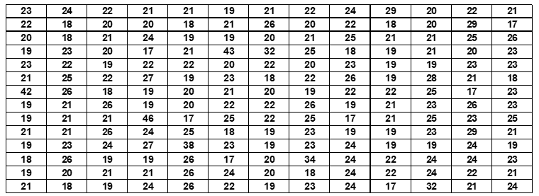
For these 182 data the mean is 22 years and the standard deviation is 4 years. The use of Gauss’s normal distribution theory for the definition of categories as described in section 2.1 results in the following categorization of the variable and its respective frequency distribution:
Table 8: Categorizatio of the age of the candidates
| Category or class name | Category or class value |
| Above the mean | > 26 (22 + 4) |
| Within the mean | 18 – 26 (22 ± 4) |
| Below the mean | < 18 (22 – 4) |
Source: Author
Table 9: Frequency distribution of the age of 182 access exam candidates.
| Age (in years) | Number of candidates | |
| Above the mean (> 26) | 13 | 7% |
| Within the mean (18 – 26) | 162 | 89% |
| Below the mean (< 18) | 7 | 4% |
Source: Author
Once the Gauss theory is applied and the frequency distribution table is constructed, its interpretation is now easy and clear to be done. The frequency distribution shows that the majority of the 182 candidates, representing 89% of them, are 18 to 26 years of age and considered candidates with an age within the mean. The percentage of candidates above and below the average is comparatively residual, being 7% and 4% respectively. This information is of great importance to the management of the University that can make the best use of it for what it deems convenient.
2.2.4 FREQUENCY DISTRIBUTION USING PREDEFINED CATEGORIES
The reference values and respective categories, standardized and certified by the world scientific community through the World Health Organization (as already described in section 2.1) are used as body of the table, resulting in the following frequency distribution of Body Mass Index of candidates to the access exam in academic years of 2008 and 2009:
Table 10: BMI distribution of the sampled individuals.
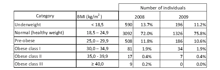
Table 10 indicates that most of the candidates both in 2008 and 2009, have normal weight. Fortunately, the number of people with class III obesity, and therefore with great health risk, is very low in 2008 and non-existent in following year.
2.2.5 USE OF PRE-DEFINED CATEGORIES VERSUS MATHEMATICAL CRITERIA IN THE CONSTRUCTION OF CLASS FREQUENCY DISTRIBUTION TABLES
It is shown below the inadequacy of the mathematical criteria for the construction of frequency distribution tables of classes for variables with predefined categories.
Consider the Body Mass Index data for the academic year 2008, a total of 4297 individuals. Looking at the criteria described in point 2.1, those that establish 6 as minimum number of categories (DAWSON and TRAPP, 2003) are coincident with the number of predefined categories for the BMI. Once the number of categories is defined, the maximum value and the minimum value must be identified to calculate the total amplitude, which in turn will be used to calculate the class interval.
Table 11: Summary statistics of the sampled data
| Sample size | 4297 |
| Maximum value | 49 |
| Minimum value | 8 |
| Amplitude (maximum – minimum) | 41 |
| Number of classes or categories | 6 |
| Class Range (Amplitude divided by the Number of Categories) | 6.8 |
Source: Author
Once the class range is determined, the limits of each of the 6 categories can be finally calculated. The lower limit of the 1st category is the minimum value and the upper limit of this category is obtained by adding the class range. The same is done for the other categories and the following result is obtained:
Table 12: Categories of the BMI and their calculated values.
| Category | BMI values | |
| 1 | 8,0 | 16,2 |
| 2 | 16,3 | 24,5 |
| 3 | 24,6 | 32,8 |
| 4 | 32,8 | 41,0 |
| 5 | 41,0 | 49,2 |
Source: Author
The table below shows a comparison between the calculated values and the predefined values.
Table 13: Comparison of the pre-defined values with the calculated values.
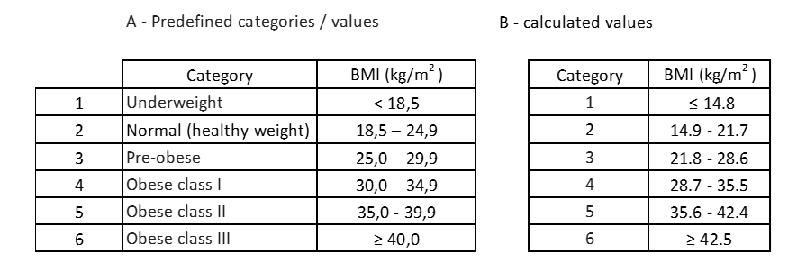
The first finding is that the calculated categories do not have their own designation, that is, they do not have attributes that qualify the condition in the individual. The second finding, despite the same number of categories, the values of each category are not equal. By the calculated categories, individuals with a BMI between 14.9 and 21.7 would be mistaken for having normal weight, when in fact some of them are in the “underweight” condition.
3. FINAL CONSIDERATIONS
Frequency distribution tables are very useful tools in data processing. Their construction must, however, comply with certain scientifically valid criteria. It is essential to ensure that, irrespective of the criterion adopted, the interpretative reading of the data leads to logical and understandable conclusions about the behavior of the variable. In this regard, the link between quantitative and qualitative attributes is crucial. Thus, the suggested criterion, based on the use of Gauss’s Normal Distribution Theory for the categorization of variables, is quite feasible.
For all that has been expressed, there is enough ground to introduce the differentiation of class frequency distribution tables into two types, that are, tables of frequencies of pre – defined classes or categories and tables of frequencies of classes or categories to be defined, suggesting thus its adoption as a concept.
REFERENCES
BEIGUELMAN, Bernardo. Curso prático de bioestatística. 5ª Edição Revisada. FUNPEC Editora, 1994.
CAQUET, René. 250 Exames de Laboratório – Prescrição e Interpretação, 10ª Edição. Rio de Janeiro: Livraria e Editora Revinter, 2011. ISBN 978-85-372-0338-5
DAWSON, Beth & TRAPP, Robert Greig. Bioestatística básica e clínica. 3ª edição. McGraw-Hill Interamericana do Brasil, 2003. ISBN 85-86804-32-0
GRUNDY, Scott M. Third Report of the National Cholesterol Education Program (NCEP) Expert Panel on detection, evaluation, and treatment of high blood cholesterol in adults (Adult Treatment Panel III). Final report. Circulation, 2002, 106:3143–3421 https://ci.nii.ac.jp/naid/10030733296/
KEYS, A., FIDANZA, F., KARVONEN, M. J., KIMURA, N., & TAYLOR, H. L. (1972). Indices of relative weight and obesity. Journal of chronic diseases 25 (6-7), 329-343.
KUZMA, Jan W. & BOHNENBLUST Stephen E. Basic Statistics for the Health Sciences. (Fourth ed.). New York: McGraw-Hill Higher Education 2001. ISBN 0-7674-1752-6
MILTON, Janet Susan. & TSOKOS, Janice Oseth. (1991). Estadistica para biologia y ciencias de la salud. Madrid: Interamericana McGraw-Hill – Madrid.
PEDROSA, Rodrigo Pinto and DRAGER, Luciano Ferreira. “Diagnóstico e classificação da hipertensão arterial sistêmica.” MedicinaNET [https://scholar.google.com/scholar] (2017).
PENA, Rodolfo F. Alves. “Como é feito o cálculo do IDH?”; Brasil Escola. Available on: https://brasilescola.uol.com.br/geografia/desenvolvimento-humano.htm. Retrieved on March 25, 2020.
REIS, Elisabeth. Estatística descritiva. Edições Sílabo, 2005. Lisboa. ISBN 972-618362-6
RICE, Kathryn and SCOTT Paul. Carl Friedrich Gauss. Australian Mathematics Teacher 61.4 (2005): 2-5.
The seventh report of the Joint National Committee on prevention, detection, evaluation, and treatment of high blood pressure. JAMA 2003; 289: 2560-72. Cited in Pedrosa and Drager (2010).
TRIOLA, Marc M. & TRIOLA, Mario F. Bioestatistics for the biological and health sciences. Boston: Pearson Education, 2006. ISBN 0-321-19436-5
WORLD HEALTH ORGANIZATION. “Obesity: preventing and managing the global epidemic.” (2000). Google Scholar
[1] PhD in Agricultural Sciences (Dr Sc Agr), Agronomist engineer.
Sent: February, 2021.
Approved: March, 2021.