ORIGINAL ARTICLE
MORAIS, Cláudio Marcelo [1]
MORAIS, Cláudio Marcelo. The imaginary unit described as an algebraic ambiguity. Revista Científica Multidisciplinar Núcleo do Conhecimento. Year 09, Ed. 03, Vol. 01, pp. 05-28. March 2024. ISSN: 2448-0959, Acess link: https://www.nucleodoconhecimento.com.br/mathematical-olympiads/imaginary-unit, DOI: 10.32749/nucleodoconhecimento.com.br/mathematical-olympiads/imaginary-unit
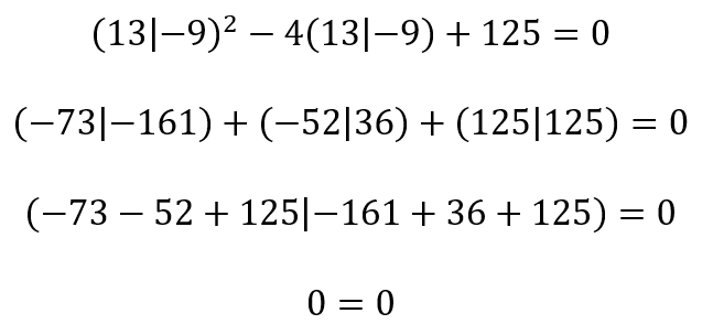
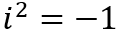
A complex number is formed by a real part and an imaginary part, the latter being composed of a real number multiplied by the imaginary unit “i,” defined as the square root of
Keywords: Imaginary numbers, Complex numbers, Complex plane, Polynomial functions.
Since their emergence in the second half of the 16th century to today, complex numbers have been important not only for mathematics but also have allowed scientists and engineers (Cayemitte, 2000) numerous applications that have helped drive scientific and technological development. Particularly in Physics, recent studies, Renou et al. (2021) and Li et al. (2022), have shown that complex numbers are indeed indispensable for expressing standard quantum theory. However, before the formal establishment of the complex number system, imaginary numbers were viewed with some suspicion by mathematicians and were initially treated only as a convenient algebraic trick to solve cubic equations where dealing with square roots of negative numbers was necessary. The origin of complex numbers is linked to the Italian mathematician Rafael Bombelli (1526-1572), whose work (Bombelli, 1572) demonstrated that manipulating
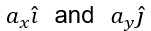
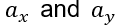
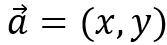
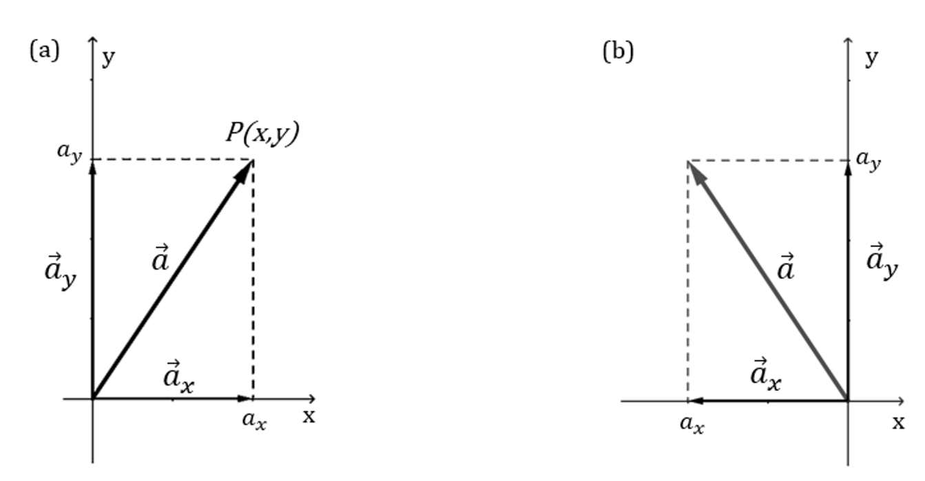
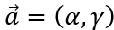
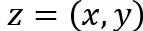
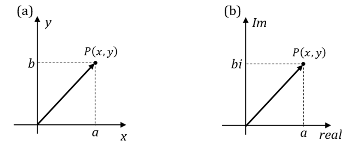
Given a vector
Fig. 1: (a) Vector
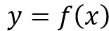
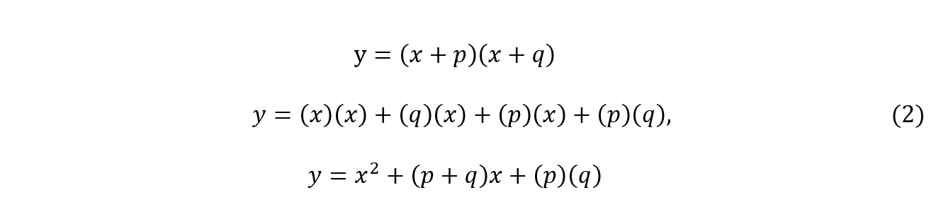
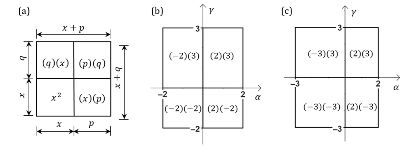
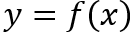
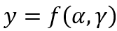
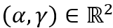
Consider the xy and αγ planes in three-dimensional Euclidean space. The xy plane will be used to plot the curve of any second-degree equation, while the αγ plane, hereinafter referred to as the “scalar plane,” will be used to represent the terms of this equation through scalar rectangles and their associated vectors. For this, let us consider the quadratic polynomial function
where p and q are real numbers. Making
Fig. 2: (a) Diagram for the quadratic function; (b) Representation of the function
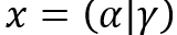
In the previous section, we saw that the variable x originates the two sides of a square scalar rectangle, referring to the quadratic term, when represented in the scalar plane. Therefore, in this plane, x occupies two dimensions, namely, one on the α axis and another on the γ axis. Thus, for any x, we have
Even though the variable x has numerically equal values on these two axes, there is an ambiguity as it simultaneously represents the two complementary components of the same vector.
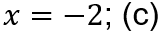
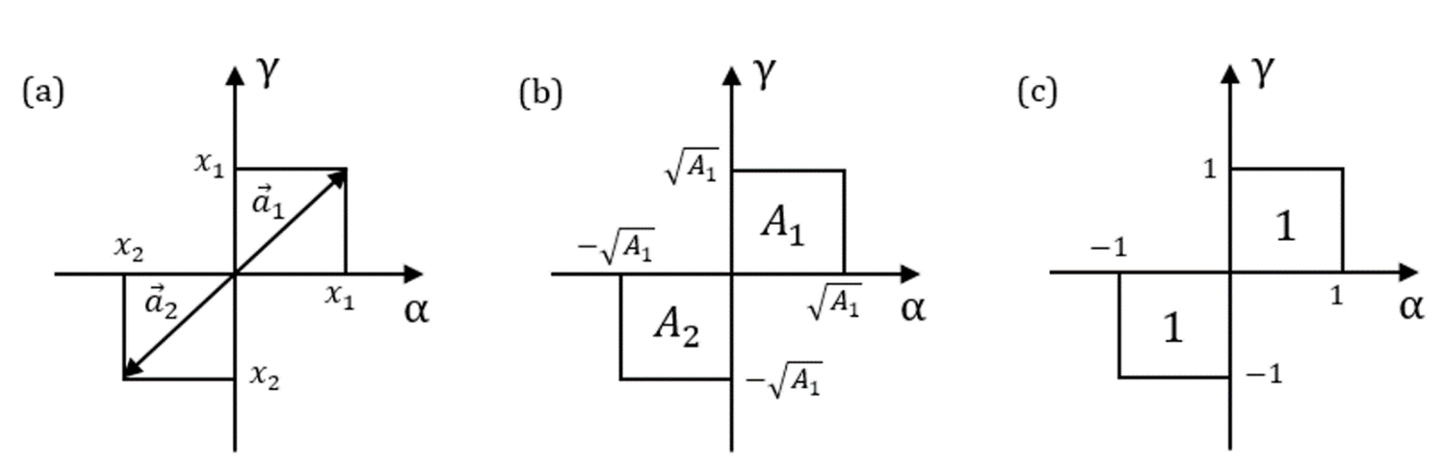
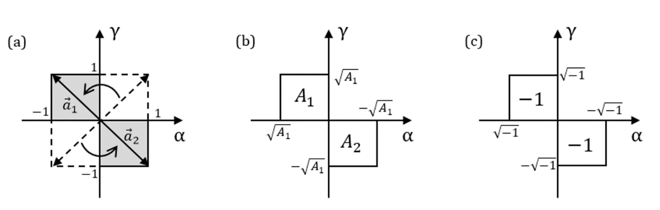
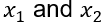
Fig. 3: (a) Case where there is one root in each odd quadrant; (b) Each square has sides with length equal to the square root of the product of the components; (c) The roots of
Now let’s see how the complementary values of x seen in the scalar plane correspond to the unique value that this variable presents in the xy plane. Note in figure 3b that each side of the square formed by the variable x has a length equal to
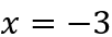
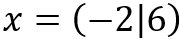
As an example, let’s do the same development for the roots
Therefore, the ambiguity that the variable x exhibits in the first and third quadrants of the scalar plane is reducible to the univocal value observed in the xy plane.
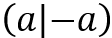
Before we proceed, let’s simplify the notation seen in (3). From this point on, we will define the following notation:
We will call this form ‘joint notation’. The expressions (4) and (5), respectively, can be written in the following joint forms:
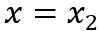
By setting x equal on both sides of each identity in (8), we have:
Let’s consider the relative positions in which the scalar components appear on each side of the equivalence seen in (7) as a canonical order to be followed. Obviously, for any real x, there will always be a combination of components
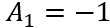
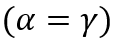
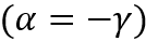
According to what has been seen so far, the positive roots of second-degree equations allow us to form rectangles in the first quadrant of the scalar plane, while the negative roots do the same in the third quadrant. However, these diagrams still do not allow us to represent roots in the form of complex numbers or even purely imaginary numbers, since the α and γ axes are real. Hence, we could inquire about the second and fourth quadrants of this plane: do they have any relation to complex numbers? To answer this question, let’s start from the roots of
Fig. 4: (a) Quadrant change by rotating the vectors by 90°; (b) The same relationships seen for the odd quadrants; (c) Scalar rectangles and their roots
So, if the root of the equation is in the second quadrant of the scalar plane, we will have α and γ equal to
To apply (10) and (11) to the ambiguity condition of the quadratic term expressed by (3), we will substitute the real values of α and γ seen in figure 4a, obtaining:
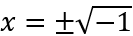
However, unlike what was done in section 3.1, it is no longer possible to apply the idempotent law of conjunction to assign a single value to the variable x; that is, in the even quadrants, the scalar components present an irreducible ambiguity. This means that there are combinations of components in the scalar plane for which there is no corresponding real number in the xy plane. However, we know that the solution
Applying the joint notation to (14) and (15), we have:
Finally, by eliminating x in (16) and (17) respectively, we get:
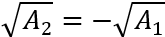
Therefore, note that the figure we obtained in 4a, by rotating the roots of
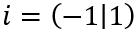
The rule for multiplying a real number by the imaginary unit can be understood as multiplying this real by a vector
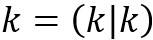
However, in joint notation,
Letting k vary from
The operation of adding two real numbers,
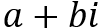
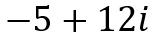
A complex number can be succinctly described as a real number added to a multiple of the imaginary unit. Thus, being a and b two real numbers and i the imaginary unit, a complex number can be algebraically represented as
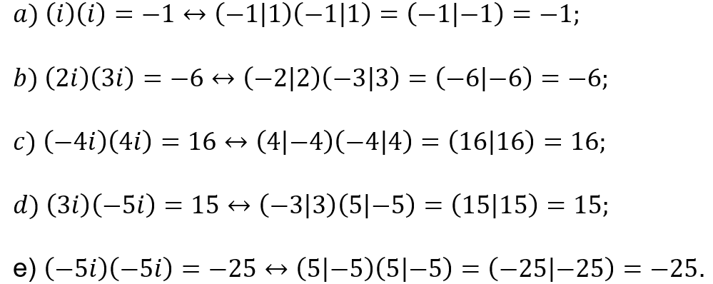
Let’s see some examples:
Therefore, in the scalar plane, a complex number represents the sum of a vector from an odd quadrant with a vector from an even quadrant. Also note that we have two ways to represent a complex number jointly: the form seen in (21) will be called the analytical joint form and the form seen in (22) will be called the synthetic joint form.
The change from a number written in algebraic form
For example, the complex number
Let’s now derive a general formula for multiplying any two numbers written in synthetic joint form. First, given two complex numbers in algebraic form
Using the transformation rule seen in (21), let’s convert only the right side of the equality in (24) to joint form:
In joint form, the product of two complex numbers can be written as:
Replacing
Thus, by direct comparison, we obtain:
Substituting the values from (28) into (25), we get:
Finally, algebraically developing the two components of the equation above and substituting
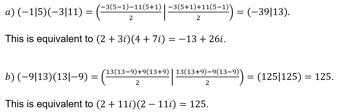
Examples:
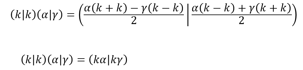
To obtain the product between a real number and a complex number in joint form, we simply do
This result agrees with equation (19), which was used to generate any imaginary number from the imaginary unit.
A good simplification can be achieved when we have two imaginaries to be multiplied. Setting
Optionally, we can eliminate the negative components of the result obtained by doing
Examples:
We can simplify formula (29) a bit by multiplying a complex number by itself. Setting
Examples:
The square of a real number can be obtained in a simplified way by making
Similarly, we can obtain the square of an imaginary number in both forms
Therefore, both the square of two real numbers and the square of two imaginary numbers can be obtained by the product of the scalar components.
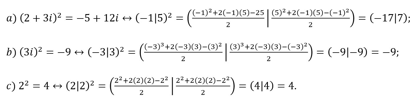
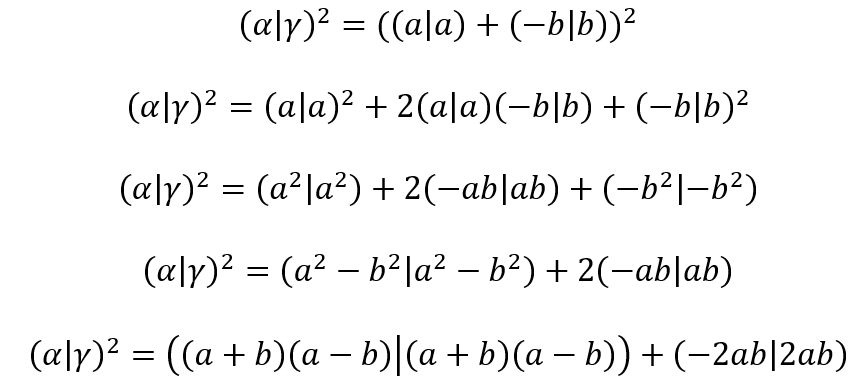
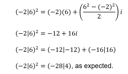
Given
Finally, writing the result in algebraic form, we find that:
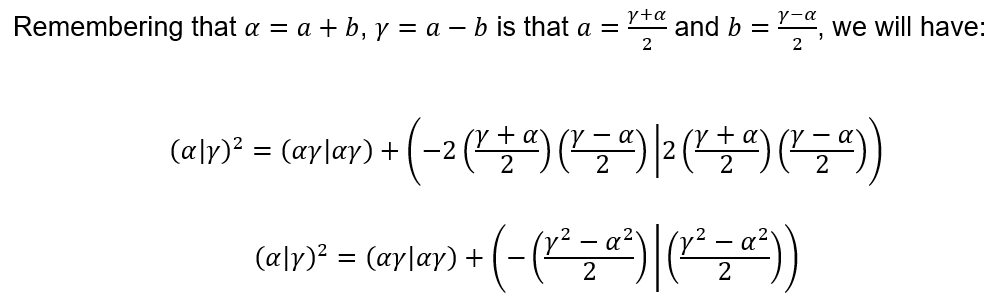
This result shows us that when we square a complex number, we obtain as a result the product of the scalar components plus an imaginary term, which can be described as half the difference of the squares of the components. Therefore, if
Example:
Given
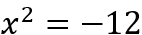
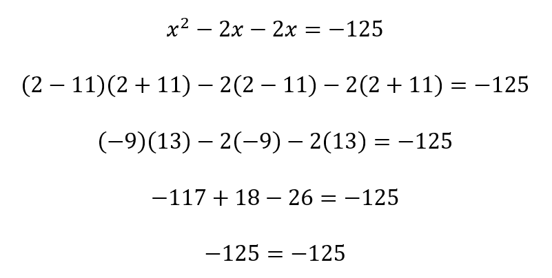
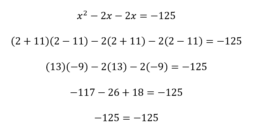
Let’s now verify the graphical solutions in the real plane for second-degree equations with negative roots. For this, let’s take as an example the equation
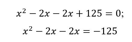
The first step is to write this equation in the form of scalar products, similar to what was seen in section 2.2, and then separate the independent term, as follows:
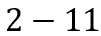
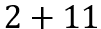
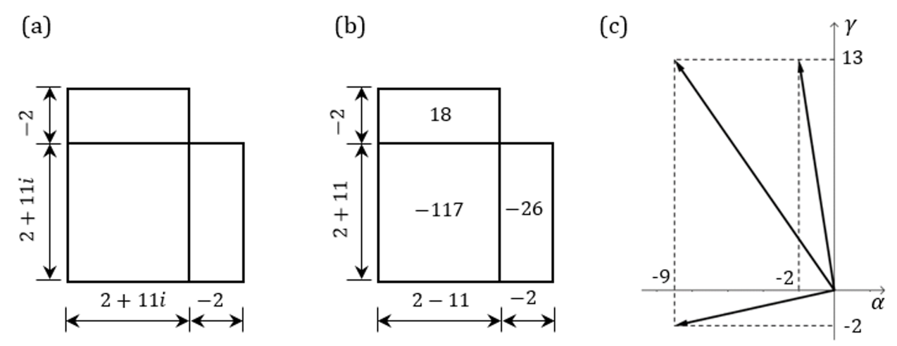
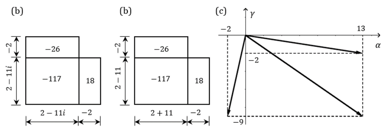
The independent term is nothing more than the product of the two roots, and its calculation was already seen in example b of section 6.1. The part on the left side of the equality allows us to obtain the diagram in figure 5a. In the diagram in figure 5b, we write
Fig.5: (a) Diagram for
In figure 5c, we can see the combination of vectors in the scalar plane representing the equation
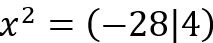
Substituting
In figures 6a and 6b are the scalar diagrams made from
Fig.6: (a) Diagram for
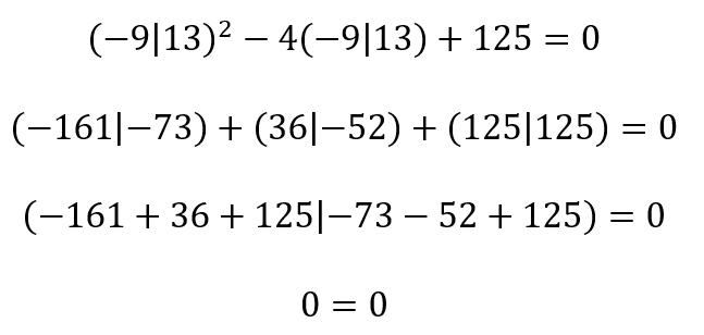
Another way to verify the roots of a second-degree equation without using imaginary numbers is to simply replace the algebraic form with the joint form. Returning to the equation
Similarly, substituting the second root into the given equation, we have:
The basic difference between the two verification methods presented is that, in the first method, although the variable x takes on different values due to its ambiguous nature, each occurrence of x in the equation corresponds to a real and univocalvalue, following the diagram used as a reference. In the second method, the notation itself and the appropriate rules of algebraic manipulation already carry within them the ambiguous nature of the variable, so that every occurrence of x can always correspond to the same pair of scalar components. This second way of working with complex numbers, as we have seen, is completely equivalent to the algebraic form
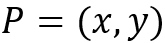
Complex numbers can be defined as ordered pairs
Fig.7: (a) Plane in
Therefore, the use of the scalar plane to represent complex numbers is not merely a formal matter, but a paradigm shift that allows us to understand complex numbers as part of the real plane. Thus, it is unnecessary to establish the set of complex numbers
The imaginary unit, although it can be operated on as a number, is not a number per se, but an ambiguous quantitative notion that simultaneously represents the two unit components of a vector located in the second quadrant of a real coordinate system, such that we cannot attribute a univocal value to i: all we can assert is that
BOMBELLI, Rafael. L’algebra. Veneza: Giovanni Battista Pedrezani, 1572. 212 p.
CAYEMITTE, Fritz Isaac. Contribution of the theory of complex numbers to the field of electrical engineering education and practice. Columbia: Columbia University, 2000. 238 p.
HALLIDAY, David; RESNICK, Robert. Fundamentos de Física 1. Rio de Janeiro: LTC – Livros Técnicos e Científicos, 1991. 300 p. Tradução de Adir Moysés et al.
LI, Zheng-Da; MAO, Ya-Li; WEILENMANN, Mirjam; TAVAKOLI, Armin; CHEN, Hu; FENG, Lixin; YANG, Sheng-Jun; RENOU, Marc-Olivier; TRILLO, David; LE, Thinh P. Testing Real Quantum Theory in an Optical Quantum Network. Physical Review Letters, [S.L.], v. 128, n. 4, p. 4-28, 24 jan. 2022. American Physical Society (APS). http://dx.doi.org/10.1103/physrevlett.128.040402.
LIPSCHUTZ, Seymour. Teoria dos Conjuntos. São Paulo: McGraw-Hill do Brasil, 1972. 337 p. Tradução de Fernando Vilain Heusi da Silva.
MOLTER, Alexandre et al. Trigonometria e números complexos: com aplicações. São Paulo: Edgard Blücher Ltda, 2020. 312 p.
NAHIN, Paul J.. An imaginary tale: the story of [the square root of minus one]. Princeton: Princeton University Press, 1998. 297 p.
RENOU, Marc-Olivier; TRILLO, David; WEILENMANN, Mirjam; LE, Thinh P.; TAVAKOLI, Armin; GISIN, Nicolas; ACÍN, Antonio; NAVASCUÉS, Miguel. Quantum theory based on real numbers can be experimentally falsified. Nature, [S.L.], v. 600, n. 7890, p. 625-629, 15 dez. 2021. Springer Science and Business Media LLC. http://dx.doi.org/10.1038/s41586-021-04160-4.
[1] Specialization in Instrumentation and Process Control from the National Service for Industrial Apprenticeship-SENAI; Professional qualification as an Electronics Technician from the Instituto Monitor S/C Ltda. Graduated in Physics from the Federal University of Minas Gerais. ORCID: 0009-0001-4633-3914. Currículo Lattes: http://lattes.cnpq.br/9333737637565760.
Material received: December 26, 2023.
Material approved by peers: January 16, 2024.
Edited material approved by authors: February 23, 2024.
In Papillary Thyroid Carcinoma (PTC), the BRAFV600E mutation represents 90% of cases, considered a point…
Introduction: Osteoporosis and cardiovascular diseases are frequent diseases, with high morbidity and mortality, and occur…
Introduction: Hepatocellular Carcinoma (HCC) is a primary liver neoplasm and the fastest-growing cause of cancer-related…
Background: Kombucha is the fastest growing product in the beverage market and one of the…
This study was conducted in two public squares in the city of Rio de Janeiro:…
This paper presents a historical and technical analysis of the development of software based on…